Time-Series-Analysis

Files

Main Folder

pollution.csv - dataset of Beijing PM2.5 Metro_Interstate_Traffic_Volume.csv - dataset of traffic volume

VAR_Multivariate.ipynb - Implementation of VAR Model on 'pollution' dataset LSTM_Multivariate.ipynb - Implementation of LSTM Model on 'pollution' dataset LSTM_Multivariate_traffic.ipynb - Implementation of LSTM Model on 'trafffic' dataset FB_Prophet_Multivariate.ipynb - Implementation of FB Prophet on 'pollution' dataset

Performance_Evaluation - folder that contain performances of different algorithms

VAR_Multivariate_Performance.ipynb - Performance of VAR Model LSTM_Multivariate_Performance.ipynb - Performance of LSTM Model FB_Prophet_Multivariate_performance.ipynb - Performance of Prophet Model

Note: You can learn how algorithms work by viewing the files in the main folder You can check different performances by viewing the files in the Performance_Evaluation folder

Dataset

The raw dataset is like this:

No	year	month	day	hour	pm2.5	DEWP	TEMP	PRESS	cbwd	Iws	Is	Ir
1	2010	1	1	0	NA	-21	-11	1021	NW	1.79	0	0
2	2010	1	1	1	NA	-21	-12	1020	NW	4.92	0	0
...	...	...	...	...	...	...	...	...	...	...	...	...

Processed data is like this:

date	pollution	dew	temp	press	wnd_dir	wnd_spd	snow	rain
2010-01-01 00:00:00	0.0	-21	-11.0	1021.0	NW	1.79	0	0
2010-01-01 01:00:00	0.0	-21	-11.0	1020.0	NW	4.92	0	0
2010-01-01 02:00:00	0.0	-21	-11.0	1019.0	NW	6.71	0	0
...	...	...	...	...	...	...	...	...
2014-12-31 19:00:00	8.0	-23	-2.0	1034.0	NW	231.97	0	0
...	...	...	...	...	...	...	...	...

• 'pollution.csv' is the pre-processed data of Beijing PM2.5, with renamed columns. All 'NA' values are marked as 0.
• The column 'pollution' is the y value that we will use different algorithms to predict.
• 'date' is the index with one hour for each step.
• Other columns are variables that influence and decide the value of the pollution, which should be considered in the training and prediction procedure.

Note: To prepare for the training and testing, additional work need to be done

• The attribute 'wnd_dir' is string. Models only accept numerical datas, so 'wnd_dir' will be encoded which originally is in type of string.

values = df.values
encoder = LabelEncoder()
values[:, 4] = encoder.fit_transform(values[:, 4])

• In this project, 90% data is used for training and the remaining 10% data is used for testing.

Multivariate Time Series Forecast Algorithms:

Traditional methods:

1. VAR - Vector Autoregression

Tutorial:

Multivariate Time series using Vector Autoregression (VAR)

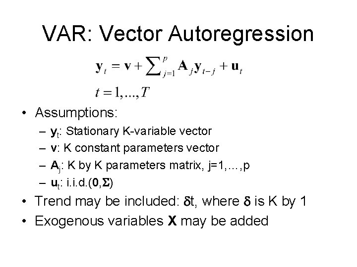
Vector Autoregression will give each past variable a weight value. In this case, we choose lag = 25, which means for past 25 steps, each variable will be assigned a weight to count for the prediction value.

Model Training

model = VAR(df_train, freq="1H")
results = model.fit(25)

As VAR can predict not only the y-value that we want, but aslo the x-values (variables) like 'dew', 'temp', etc., we can choose the prediction value we want.

Prediction

pred_next = results.forecast(df_test.values[i-25:i],steps = futureStep)[:, 0]

Since we choose lag = 25, we just feed the model with 25 past values df_test.values[i-25:i]. We can tell the model how many future values we want by giving steps = futureStep . If we set futureStep = 3, this model will next 3 hours' prediction of pollution.

VAR-RMSE

To test RMSE (Root Mean Square Error) of the model, we use 10% of dataset. For example, we set futureStep = 5, then we use df_test.values[0:25] (25 steps' data) to predict the pollution at point [25, 30]. Then we use df_test.values[5:30] to predict the pollution at point [30, 35]...

After scan through all df_test, we compare the prediction value pred with the. ground truth df_test['pollution'] and calculate the RMSE value for futureStep = 5. All are the same for other future steps.

VAR-Prediction

Machine Learning methods:

1. LSTM - Long Short-term Memory

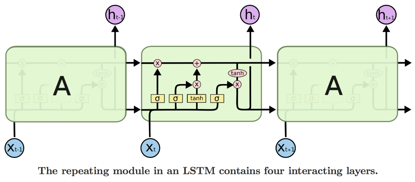
Tutorial:

Multivariate Time Series Forecasting with LSTMs in Keras

Data Preparation

Different from VAR, the dataset should be first reframed as: || var1(t-1) | var2(t-1) | var3(t-1)|... |var7(t-1) | var8(t-1) | var1(t) | |--|--|--|--|--|--|--|--|--|--|--|--|--| |1|0.0|0.279412|0.131148|...|0.0|0.0|0.0| |2|0.0|0.279412|0.114754|...|0.0|0.0|0.0| | ... |...|...|...|...|...|...|...|...|...|...|...|...|

Here, we aggregate variable and 'pollution' of past 1 step as variables to train. Later when implementing LSTM, we choose pastSteps = 24 and futureSteps = 5, and hence there are 24*8 attributes of variables + var1(t) + var2(t) + var3(t) + var4(t) + var5(t)

We can reframe the dataset by using function: series_to_supervised(data, n_in=1, n_out=1, dropnan=True)

data is the dataset you need to process, n_in is the number of past steps used to train. (in time series forecasting, the past output is also the variable). n_out is the number of future values that we want to predict. e.g. futureStep = 5 pastStep = 24 The reframed data has the attributes of:

var1(t-24)	var2(t-24)	...	var8(t-24)	var1(t-23)	...	var8(t-23)	var1(t-22)	...	var1(t-1)	...	var8(t-1)	var1(t)	var1(t+1)	...	var1(t+4)

Note: You need to put the output in the first column of the dataset so that the var1 could be the prediction variable. e.g. 'pollution' is the first column in our case.

date	pollution	dew	temp	press	wnd_dir	wnd_spd	snow	rain

Model Training

model = Sequential()
model.add(LSTM(50, input_shape=(train_X_reshape.shape[1], train_X_reshape.shape[2])))
model.add(Dense(futureStep)) # dense layer will give the output number referring to the futureStep
model.compile(loss='mae', optimizer='adam')

epochs = 50 # modify here to choose training epoches
model.fit(train_X_reshape, train_y, epochs=epochs, batch_size=72, validation_data=(test_X_reshape, test_y), verbose=0, shuffle=False, )

The train_X_reshape and test_X_reshape are given by:

# reshape input to be 3D [samples, timesteps, features]
train_X_reshape = train_X.reshape((train_X.shape[0], 1, train_X.shape[1]))
test_X_reshape = test_X.reshape((test_X.shape[0], 1, test_X.shape[1]))

Prediction

result = model.predict(test_X_reshape)

The dimensions of each array are:

pastStep: 24  futureStep: 5   train X: (39416, 1, 192)   train y:  (39416, 5)   test X: (4000, 1, 192)   test y: (4000, 5) prediction shape: (5, 4000)

RMSE

LSTM-Prediction

2. Facebook Prophet

Tutorial:

Time Series Forecasting with Facebook Prophet and Python in 20 Minutes

Multivariate Time Series Modeling using Facebook Prophet

Data Preparation

Different From LSTM, reframed data should have only one attribute of y and should be append with ds. var1(t) is named as var1(t) and date is named as ds.

The format is like:

var1(t-24)	var2(t-24)	...	var8(t-24)	var1(t-23)	...	var8(t-23)	var1(t-22)	...	var1(t-1)	...	var8(t-1)	y	ds

y and ds are the requirement of FB Prophet, fr the reference of model.

Model Training

model = Prophet(interval_width=0.95)

names = list()
for i in range(pastStep, 0, -1):
  names += [('var%d(t-%d)' % (j + 1, i)) for j in range(8)]

for variable in names:
  model.add_regressor(variable)

model.fit(train)

All variables are considered as the regressor.

Prediction

m.predict(test_temp)['yhat']

Prophet can only predict one y value for each row, named yhat. Therefore, if we want to predict more than one steps, we need to predict all next variables and next y, reframed them to var1(t-1) to var8(t-1) and then feed to the model to predict the second y.

RMSE

Prediction

Performance