ECE-666: AOMML Programming Assignment

This repository contains PyTorch implementations and Jupyter notebooks for a variety of recent optimization algorithms in deep learning, including:

• First-order methods: SGD, SGD w/ Momentum, SGD w/ Nesterov Momentum
• Adaptive methods: RMSprop, Adam, Nadam, RAdam, RAdamW, AdamW, ADADELTA, AdaBound
• Regularized and decoupled methods: SGDW, Adam w/ L2, Gradient Noise, Gradient Dropout, Learning Rate Dropout
• Higher-order enhancements: Lookahead, Aggregated Momentum

All of these components are designed to be mix-and-match, so you can—for example—train a model with RAdamW + Nesterov Momentum + Gradient Noise + Lookahead in a single run.

---

📚 Related Papers

As part of the AOMML course reading group, we have implemented and experimented with the following key papers:

1. An Overview of Gradient Descent Optimization Algorithms
2. Optimization Methods for Large-Scale Machine Learning
3. On the Importance of Initialization and Momentum in Deep Learning
4. Aggregated Momentum: Stability Through Passive Damping
5. ADADELTA: An Adaptive Learning Rate Method
6. RMSprop
7. Adam: A Method for Stochastic Optimization
8. On the Convergence of Adam and Beyond
9. Decoupled Weight Decay Regularization (AdamW)
10. Incorporating Nesterov Momentum Into Adam
11. Adaptive Gradient Methods with Dynamic Bound of Learning Rate (AdaBound)
12. Lookahead Optimizer: k Steps Forward, 1 Step Back
13. Adding Gradient Noise Improves Learning for Very Deep Networks
14. Learning Rate Dropout
15. …and more in the papers/ folder.

---

🛠 Installation

git clone https://github.com/shubhampundhir/aomml-optim-ece666.git
cd aomml-optim-ece666
conda create -n aomml-env python=3.9
conda activate aomml-env
pip install -r requirements.txt

How to run

You can run the experiments and algorithms by calling e.g.

python main.py -num_epochs 30 -dataset cifar -num_train 50000 -num_val 2048 -lr_schedule True

Key flags:

--optimizer: sgd, momentum, nesterov, rmsprop, adam, nadam, adamw, radam, radamw, adabound, adadelta, …

--lr: initial learning rate (η)

--momentum: momentum coefficient (μ) for applicable methods

--weight_decay: weight‐decay factor for SGDW / AdamW / RAdamW

--noise_std: standard deviation for gradient noise

--dropout_rate: dropout probability for gradients or learning‐rate updates

--lookahead_k, --lookahead_alpha: Lookahead steps and blending factor

--lr_schedule: enable cosine/step learning‐rate schedule

Run python main.py --help to see all options.

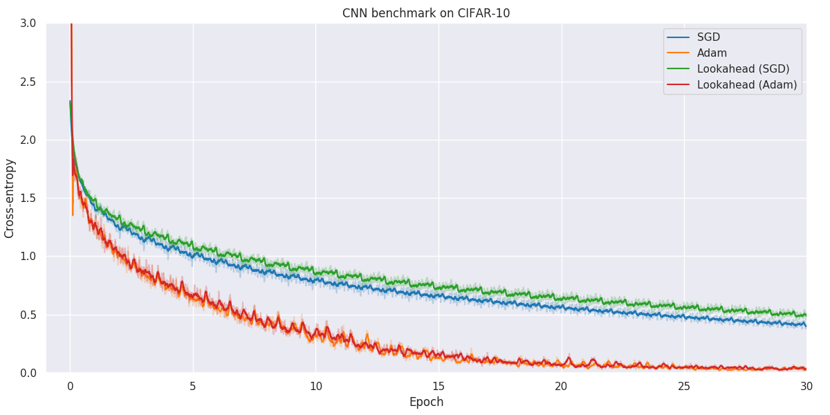
with arguments as specified in the main.py file. The algorithms can be run on two different datasets, MNIST and CIFAR-10. For MNIST a small MLP is used for proof of concept, whereas a 808,458 parameter CNN is used for CIFAR-10. You may optionally decrease the size of the dataset and/or number of epochs to decrease computational complexity, but the arguments given above were used to produce the results shown here.

---

2. Within JupyterLab

We provide four interactive notebooks:

aomml-CustomOptim-MNIST.ipynb
aomml-CustomOptim-CIFAR10.ipynb
aomml-CustomOptim-CIFAR100.ipynb
aomml-PytorchOptim-CIFAR10.ipynb

Each notebook covers:

1. Environment Setup

• In the first cell:

!pip install -r requirements.txt

2. Dataset Loading

• MNIST: transforms, DataLoader

• CIFAR-10/100: normalization, augmentations

• Model Definition

• Small MLP for MNIST

• Standard CNN (≈808k parameters) for CIFAR

3. Optimizer Configuration

• Select from custom vs. built-in optimizers

• Set hyperparameters via widget or variables

To launch:

jupyter lab

then open and “Run All” in your chosen notebook

Accuracy Metrics:(Optimizer-wise)

CNN (CIFAR-10)

MLP (MNIST-dataset):

Results

Below you will find our main results. As for all optimization problems, the performance of particular algorithms is highly dependent on the problem details as well as hyper-parameters. While we have made no attempt at fine-tuning the hyper-parameters of individual optimization methods, we have kept as many hyper-parameters as possible constant to better allow for comparison. Wherever possible, default hyper-parameters as proposed by original authors have been used.

When faced with a real application, one should always try out a number of different algorithms and hyper-parameters to figure out what works better for your particular problem.

CNN (CIFAR-10)

MLP (MNIST-dataset):