Lending Club is an online personal loan provider who provided data about rejected and approved loans for developers and lenders to utilize. Kaggler's have also utilized the datasets for competitions. I utilized a Lending Club dataset containing data for loan approvals and rejections from 2007 through 2018 provided on Kaggle by Kaggler: wordsforthewise, with the data dictionary provided by Kaggler: JonChan2003.
These data are interesting for relating rejected and approved loan candidates. If meaningful distinctions can be found between features of rejected and accepted loans, perhaps those features can be used to predict who will be accepted or rejected for loans in the future, enabling one as an investor to make better investing decisions than can be achieved by simply flipping a coin! The first stage is to find meaningful differences between groups of features.
The data from 2007 to 2018 exist in two files: One file contains the approved loans. The other file contains the rejected loans application data. The breakdown of the number of records and features can be seen in table 1.
| Table | n-Columns | n-Rows |
|---|---|---|
| Accepted | 151 | 2,260,702 |
| Rejected | 9 | 27,648,742 |
Table 1: Breakdown of datasets.
The common columns between the two datasets are as follows:
| Common Features | Datatype | Name in Accepted | Name in Rejected | NaN Count in Accepted | NaN Count in Rejected |
|---|---|---|---|---|---|
| Amount | Float | Amount Requested | loan_amnt | 34 | 0 |
| Risk Score | Float | fico_range_low, fico_range_high | Risk_Score | 33, 33 | 18,497,630 |
| DTIR | Float | dti | Debt-To-Income Ratio | 1744 | 0 |
| Years Employed | Float | emp_length | Employment Length | 146,940 | 951,355 |
| Zip code | Object | zip_code | Zip Code | Unk | Unk |
| State | Object | addr_state | State | Unk | Unk |
Table 2: Shared features between the datasets and potential targets of analysis.
Of the above features between both datasets, I was drawn to Amount, Years Employed, and Debt-to-Income Ratio (DTIR).
I hypothesize that (1) Loan amount requested for $20k and above will be approved significantly differently than for $20k and below. The null hypothesis is that lendees will have the same proportion of approved loans regardless of whether they requested loans in the $20k and above category or below $20k category.
In addition, I hypothesize that (2) lendees with 10 or more years of employment, will, on average, tend to have a significantly different number of loans approved than lendees with less than 10 years of employment history. The null hypothesis is that there is no difference between those with ten or more years of employment history and those with less in their frequency of loan approvals.
Finally, DTIR should be directly related with loan rejections. Specifically, I hypothesize that a DTIR of 0.3 or less will have significantly different proportion of loan approvals than the group with higher than 0.3 DTIR. The null hypothesis here is that the 0.3% and below group will not be statistically different from the greater than 0.3% DTIR group in loan approvals.
The goal in this EDA was to describe the three columns adequately for hypothesis testing, to draw conclusions from data. During EDA, it was discovered that DTIR was partially truncated at -1, and 100%, and the rejected loans dataset is tailing heavily to the right, with ~4% of the data above 100%, ~4.8% of the data truncated right at 100%, and roughly 5% of the data truncated at -1. Approximately 86% of data are between 0 inclusive to 100% non inclusive. The data dictionary failed to explain what those truncated values and values above the right partial truncation meant, so these data were avoided in further analysis. Thus, hypothesis 3 was not addressed in this analysis given that ~14% of data for rejected loans would have to be thrown out.
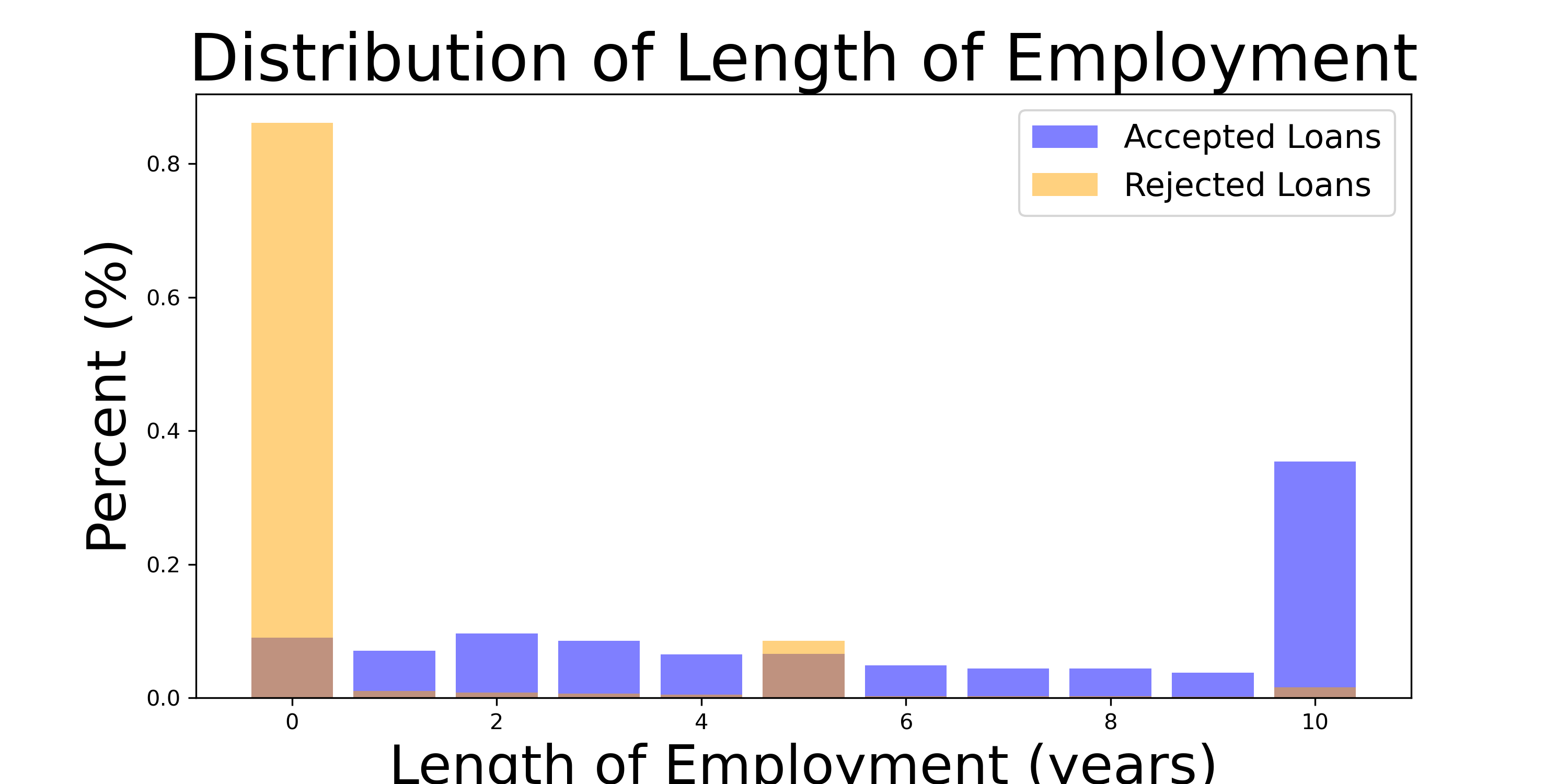
Length of employment is a binomial variable - essentially an 11 sided die, with sides representing 0 through 9 years of employment history, and a final side for 10 or more. The histogram of Employment Length looks as follows:
Figure 1: Histogram of employment length by percent illustrates difference in tendency to reject loanees with no job experience and a tendency to prefer loanees with ten or more years of experience. This ten year tendency may be cultural or selection bias from the lender.
While there appears to be a tendency to reject loans for those without experience, this makes sense. Less clear is whether the summed accepted loans for all categories up to 9 will overpower the category for 10 and above. It seems as though there is a peak at two years, and accepted loans falls off as years increases, where the truncated category at 10+ could be a sum of ever smaller values per year.
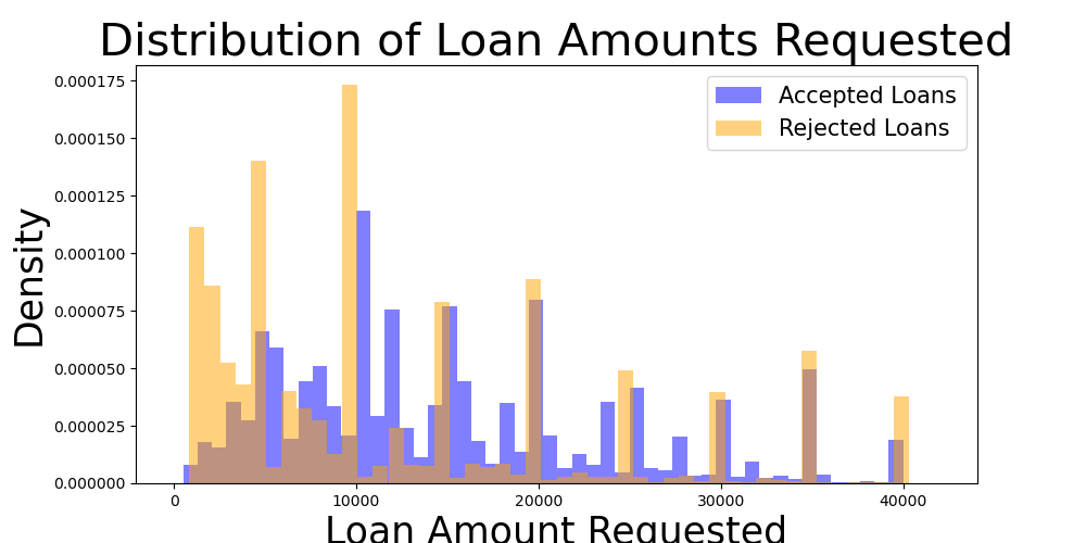
Loan Amount is theoretically a continuous variable. However, evident from the histogram is that there are striations at whole numbers where consumers have a stronger tendency to apply for loans at. Take a look at Figure 2.
Figure 2: The density plot of loan amount requested shows a tendency for consumers to apply at $5,000 increments above $10K.
Figure 2 seems to show a higher density of rejected loans below $10k. Also, the bulk of the density seems to be below $20k for both rejected and approved loans.
In order to investigate the two hypothesized groups, the successes (approved loans) at 9 and below were assembled and compared to the approved loans at the category 10+; and the successes (approved loans) at $20k and above were compiled against the successes below $20k to form two groups.
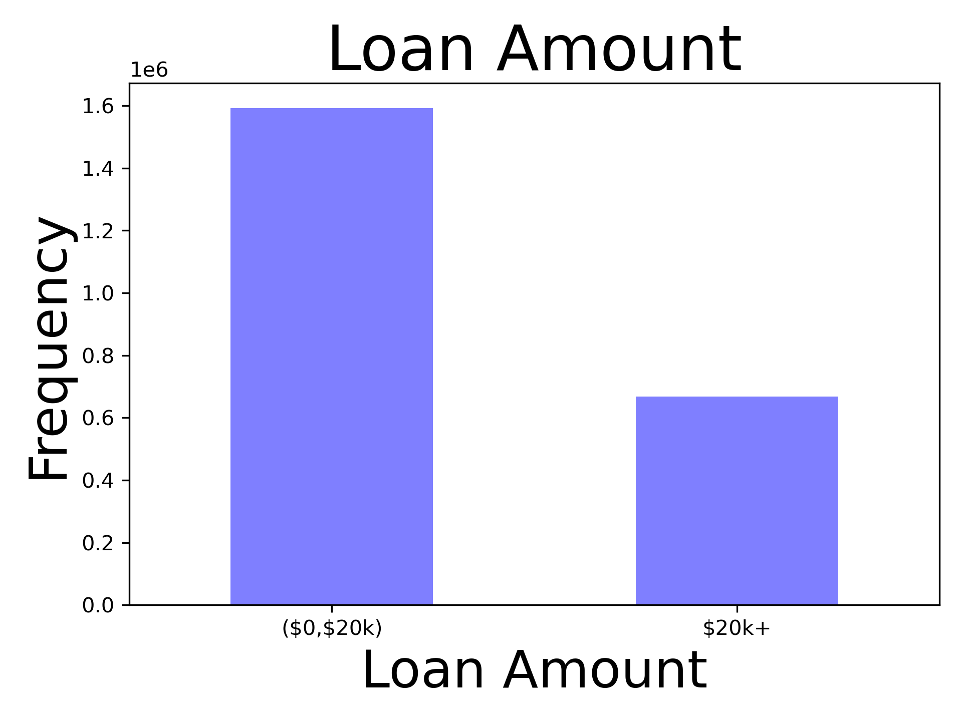
Binomial plots seem to be trending differently from each other and may be significantly different. See figures 3 & 4.
Each group was tallied, receiving a 1 if approved for a loan, and a zero if rejected for a loan. A Welch two sample t-test was conducted over a z-test due to not knowing the population variance.
For work history, the t-value for the difference in proportions is 605.41, with a p-value 0f 0.0. The p-value is smaller than the a-priori chosen critical alpha value of 0.01 so we reject the null hypothesis that the group with a work history of 10 or more years is the same as the group with a work history of less than 10 years, in favor of the hypothesis that the groups are different. The figure shows the direction of the effect.
For Loan Amount, the t-value for the difference in proportions is 952.84, with a p-value of 0.0. The p-value is smaller than the a-priori chosen critical alpha value of 0.01 so we reject the null hypothesis that the group that applied for loans of $20k or more is the same as the grouop that appied for loans of less than $20k, in favor of the hypothesis that the groups are different. The figure shows the direction of the effect.
These particular cutoffs may be useful as features in machine learning models down the road, or to inform financial analysts further in loan approval decisions. One problem with these data for loan amount is the striations. There is more probability for a loan to fall on multiples of $5k values than other values. This may have an impact on the validity of the analysis.
Feedback recieved about this analysis include the following:
-
The appropriate test is an approximate test of differences in population proportions, being the z-test. In response I show that the results of the t-test and the z-test are nearly equivalent for these data, which supports the findings regardless of which test is used. However, it wouldn't hurt to further use a more conservative adjustment to the degrees of freedom given the imbalance between the groups.
-
There was a question during a presentation about the axes of figure 3 & 4. The axes on figures 3 and 4 are not scaled but raw proportions in 1e6 units. The units were auto chosen by the grapher. The units are printed above the axis, albiet obveously difficult to see otherwise there would have been no reason for the question. I have played around with fontsize, however, I have not been successful at changing it.
-
The plot titles and axis labels were partially cut off in the original plots. I have found a workaround.
from matplotlib import rcParams
rcParams.update({'figure.autolayout': True})
For an update and formal responses to feedback, with data, and a list of feedback not yet responded to, see the slide deck.


