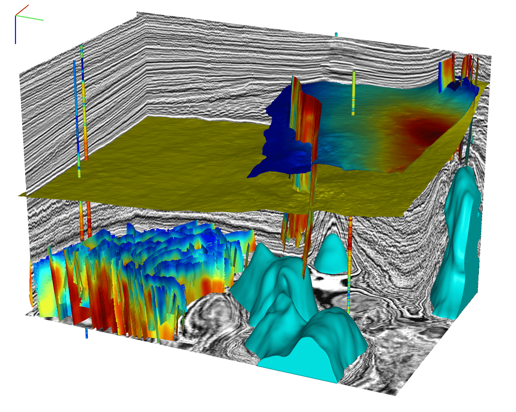
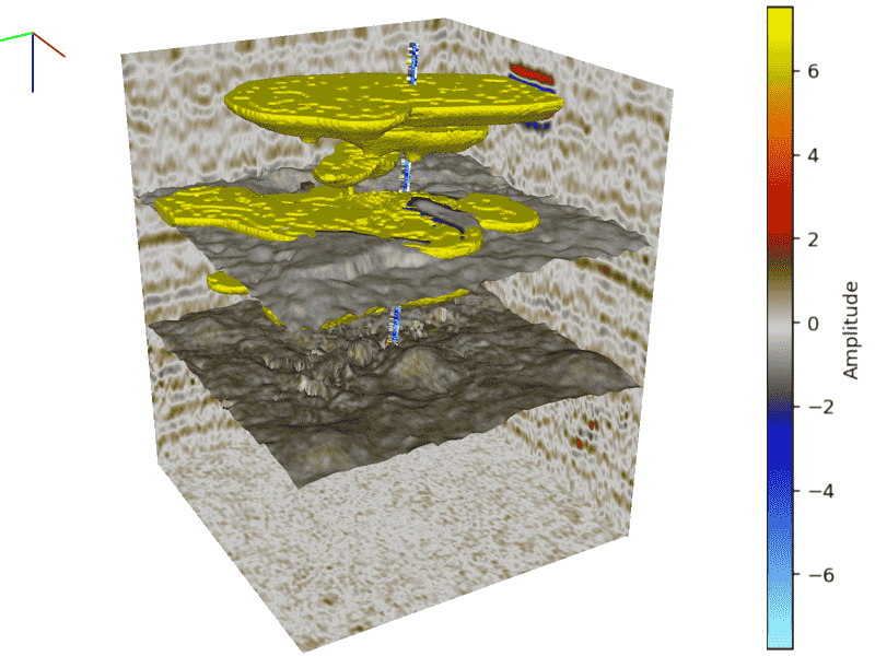
cigvis is a tool for visualizing multidimensional geophysical data, developed by the Computational Interpretation Group (CIG). Users can quickly visualize data with just a few lines of code.
cigvis can be used for various geophysical data visualizations, including 3D seismic data, overlays of seismic data with other information like labels, faults, RGT, horizon surfaces, well log trajectories, and well log curves, 3D geological bodies, 2D data, and 1D data, among others. Its GitHub repository can be found at github.com/JintaoLee-Roger/cigvis, and documentation is available at https://cigvis.readthedocs.io/.
cigvis leverages the power of underlying libraries such as vispy for 3D visualization, matplotlib for 2D and 1D visualization, plotly for Jupyter environments (work in progress), and viser for web-based visualization (SSH-Friendly). The 3D visualization component is heavily based on the code from yunzhishi/seismic-canvas and has been further developed upon this foundation.
To install via PyPI, use:
# Minimal installation
pip install cigvis

# include plotly
pip install "cigvis[plotly]"

# include viser
pip install "cigvis[viser]"

# install all dependencies
pip install "cigvis[all]"
For local installation, clone the repository from GitHub and then install it using pip:
git clone https://github.com/JintaoLee-Roger/cigvis.git
# Minimal installation
pip install -e . --config-settings editable_mode=compat

# include plotly
pip install -e ".[plotly]" --config-settings editable_mode=compat

# include viser
pip install -e ".[viser]" --config-settings editable_mode=compat

# install all dependencies
pip install -e ".[all]" --config-settings editable_mode=compat- Convenient 3D geophysical data visualization.
- Ongoing development of 2D and 1D data visualization.
- Additional colormaps tailored for geophysical data.
- Rapid display of large data in OpenVDS format.
The fundamental structure of cigvis's visualization code consists of:
- Data loading
- Creating nodes
- Passing nodes to the
plot3Dfunction
For example:
import numpy as np
import cigvis

# Load data
d = np.fromfile('sx.dat', np.float32).reshape(ni, nt, nx)

# Create nodes
nodes = cigvis.create_slices(d)

# Visualize in 3D
cigvis.plot3D(nodes)
This basic code structure allows you to quickly visualize your geophysical data using cigvis. Simply load your data, create nodes, and pass them to the plot3D function as demonstrated in the example above.
Left click and drag to rotate the camera angle; right click and drag, or scroll mouse wheel, to zoom in and out. Hold <Shift> key, left click and drag to pan move. Press <Space> key to return to the initial view. Press <S> key to save a screenshot PNG file at any time. Press <Esc> key to close the window.
Hold <Ctrl> key, the selectable visual nodes will be highlighted when your mouse hovers over them; left click and drag to move the highlighted visual node. The volume slices will update their contents in real-time during dragging. You can also press <D> key to toggle the dragging mode on/off.
Press <z> to zoom in z axis, press <Z> or <Shift> + <z> to zoom out z axis.
Press <f> to increase fov value, press <F> or <Shift> + <f> to decrease fov value.
Press <s> to save a screen shot.
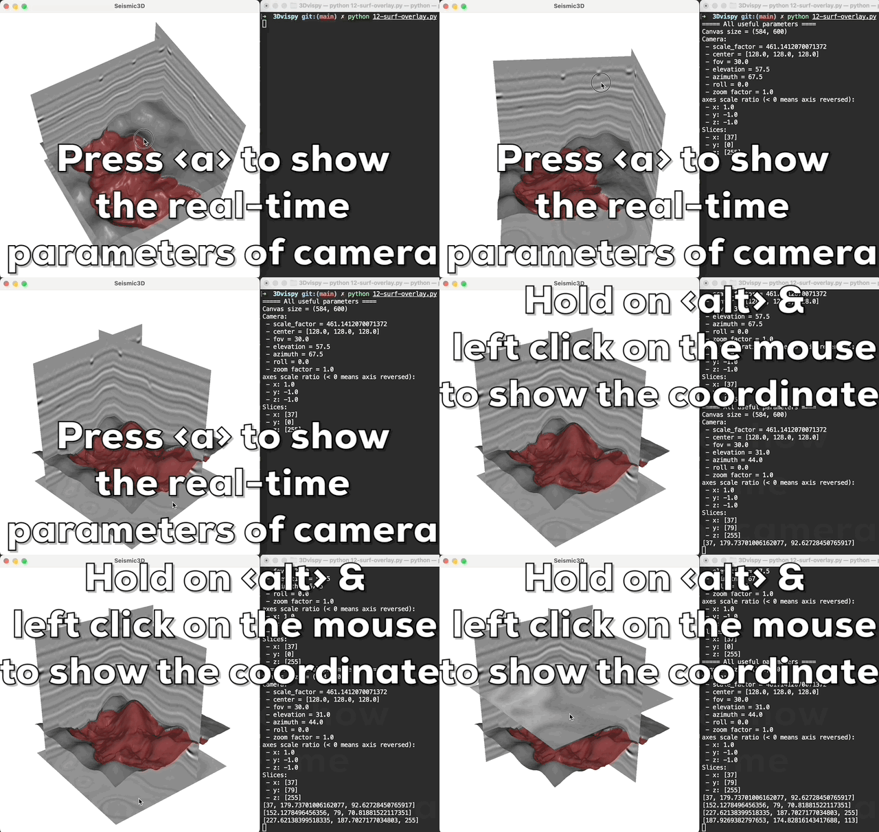
Press <a> to print the camera's parameters in real-time; hold on
the <alt> (or <option> in macos) and left click the mouse to
show the coordinate of the click point in the 3D volume.
In cigvis, we represent various geophysical data as individual nodes, assemble these nodes into a list, and then pass this list to the plot3D function for visualization.
We visualize a three-dimensional data volume as multiple slices along the x, y, and z directions. Additionally, we can overlay other three-dimensional data slices on these slices, allowing users to interactively drag them along an axis using the mouse.
Horizon data can be represented as scatter points with a shape of (N, 3), or as z-values on a regular grid of size (n1, n2).
Well log trajectories are displayed as tubes, where the size of the first well log curve is represented by the color and radius at each position along the tube. Other well log curves are displayed as surfaces attached to the tube's edge. An example is shown below (code available at cigvis/gallery/3Dvispy/09).
These capabilities within cigvis allow for versatile and interactive visualizations of a wide range of geophysical data types, enhancing the understanding and analysis of such data in geoscience applications.
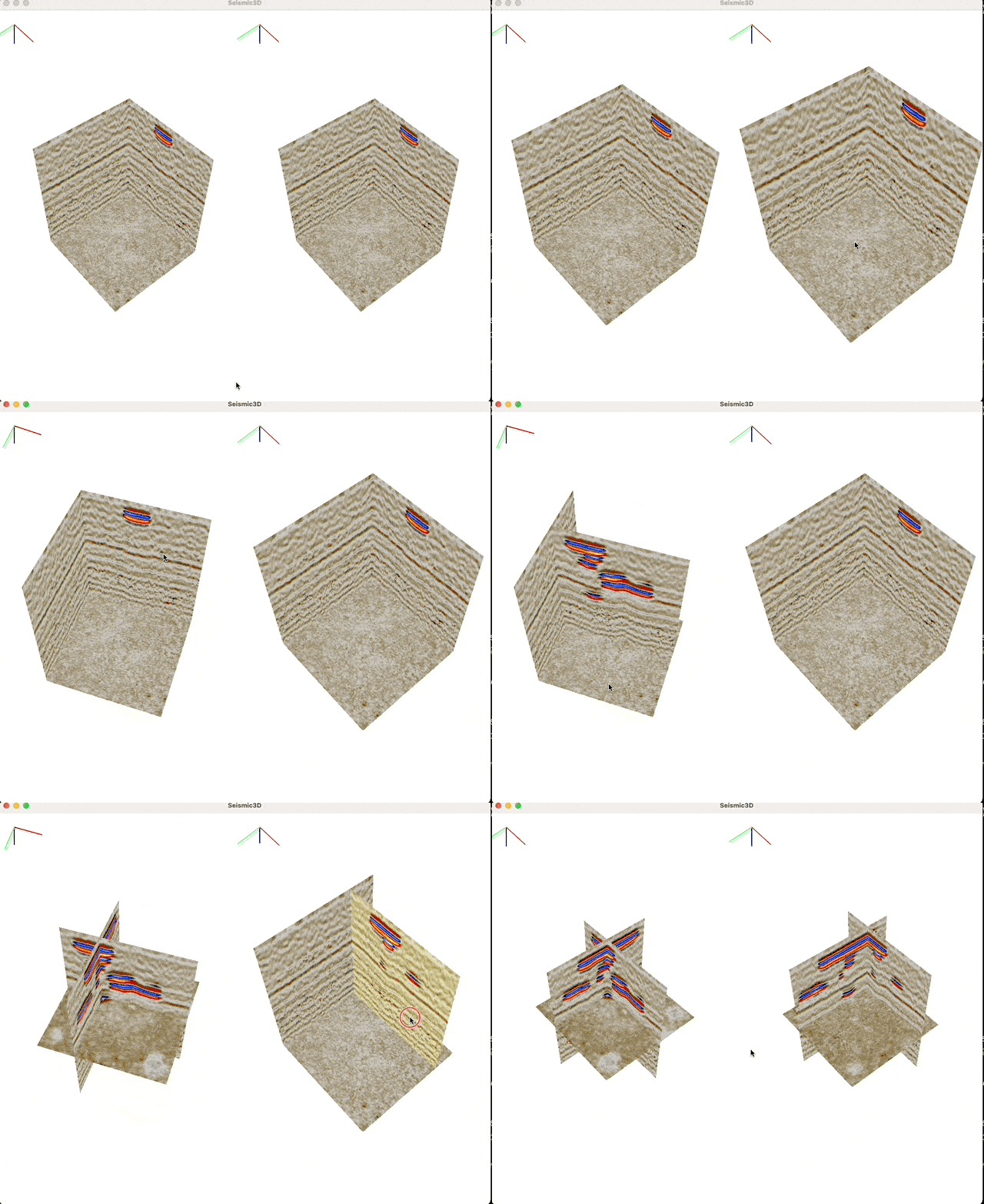
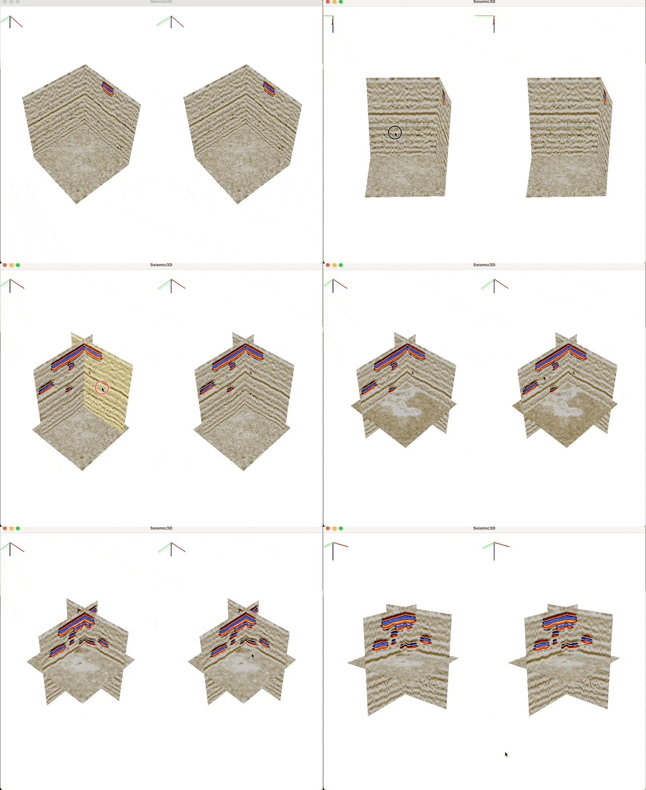
You can pass multiple independent nodes combinations to the plot3D function while specifying a grid (e.g., grid=(2,2)). This allows you to divide the canvas into multiple independent sub-canvases, where each sub-canvas displays a separate 3D data set within the same canvas. The example code for this can be found in the documentation at cigvis/gallery/3Dvispy/10.
Furthermore, you can link the cameras of all sub-canvases together (just need pass share=True to plot3D function). This means that any rotation, scaling, or slicing performed in one sub-canvas will be mirrored in all other sub-canvases, ensuring that they all exhibit the same changes simultaneously. This feature is highly advantageous when comparing multiple sets of data, such as results from different experiments, results alongside labels, seismic data compared with attributes, and more.
You can find example code for this functionality in the documentation at cigvis/gallery/3Dvispy/11.
These capabilities provide a powerful way to visualize and compare multiple independent 3D data sets within a single canvas using cigvis.
Based on viser, cigvis also supports visualization 3D data in web/browser environment with just a few lines changed. All you need to do is simply replace cigvis with viserplot, see follows:
    import numpy as np
    import cigvis
+   from cigvis import viserplot

    # Load data
    d = np.fromfile('sx.dat', np.float32).reshape(ni, nt, nx)

    # Create nodes
-   nodes = cigvis.create_slices(d)
+   nodes = viserplot.create_slices(d)

    # Visualize in 3D
-   cigvis.plot3D(nodes)
+   viserplot.plot3D(nodes)
When you are in jupyter environment, we recommand to maintain a unique server, otherwise the port will be changed.
    import numpy as np
    import cigvis
+   from cigvis import viserplot
+   server = viserplot.create_server(8080)

    # Load data
    d = np.fromfile('sx.dat', np.float32).reshape(ni, nt, nx)

    # Create nodes
-   nodes = cigvis.create_slices(d)
+   nodes = viserplot.create_slices(d)

    # Visualize in 3D
-   cigvis.plot3D(nodes)
+   viserplot.plot3D(nodes, server=server)
After calling viserplot.plot3D, it will generate some logs like:
╭─────────────── viser ───────────────╮
│             ╷                       │
│   HTTP      │ http://0.0.0.0:8080   │
│   Websocket │ ws://0.0.0.0:8080     │
│             ╵                       │
╰─────────────────────────────────────╯
If you are running the code on your local machine, just open 0.0.0.0:8080 in your browser to see the image. If you are running the code on a remote server (yes, cigvis also works when connected remotely using ssh!), you can enter {ip}:8080 in the browser to see the visualization (ip is the ip of remote server, e.g., 222.195.77.88:8080).
There are sevreal examples in examples/viser/ for reference.
All data used by examples in the gallery can be download at https://rec.ustc.edu.cn/share/19a16120-5c42-11ee-a0d4-4329aa6b754b, password: 1234.
See: cigvis/gallery
- move all functions for triangle mesh creation to
meshs/
