miniRT

miniRT render of this scene.

This project is a collaboration between:

• Natalie: Responsible for the .rt file parser.
• Alex: Focused on MiniLibX integration, ray-object intersections, shading & shadowing, and this README.

---

Overview

• How to Use: Building miniRT and defining scene elements in .rt files.
• Introduction to Ray Tracing
• Ray-Object Intersection: Mathematical definitions of object surfaces and functions for finding intersections.
  • Ray Equation
  • Quadratic Equation
  • Plane Intersection
  • Sphere Intersection
  • Cylinder Intersection
  • Finding Intersections with Objects
• Camera Ray: Computing the direction of camera rays and transforming them into world space.
• Shadow Ray: Check if the intersection point is in shadow by verifying if the light source is blocked.
• Shading: Calculate the color at the intersection point based on its surface properties and its orientation relative to the light source.
  • Phong Reflection Model
  • Diffuse Shading
  • Specular Reflection
  • Combining Shading Components

---

How to Use

1. Clone the repository and navigate into the project directory:

   git clone https://github.com/Busedame/miniRT miniRT && cd miniRT
   

2. Build the project:

• Without specular highlighting and light fading:

  make
  

• With specular highlighting and light fading:

  make bonus
  

3. macOS Users: Install X11 via XQuartz if needed:

   brew install xquartz
   

   If Homebrew is not installed, first run:

   /bin/bash -c "$(curl -fsSL https://raw.githubusercontent.com/Homebrew/install//install.sh)"
   

   After installation, restart your Mac or run:

   export DISPLAY=:0
   

4. Run the program following the instructions in the output.

The Makefile automatically detects your OS and selects the correct MiniLibX library for compilation. MiniLibX is a simple graphics library for creating windows, handling pixel coloration, and managing events.

---

Ray Tracing Files (.rt files)

Our miniRT implementation uses a left-handed coordinate system, meaning that increasing values of x move an object to the right, y moves it up, and z moves it away from the camera. The .rt files define the elements and configurations for the scene to be rendered:

Mandatory Elements

• Ambient Light
  

  • Identifier: A
  • Ambient lighting ratio (brightness) [0.0, 1.0]: 0.2
  • Color in RGB [0, 255]: 255, 255, 255

• Camera
  

  • Identifier: C
  • Position (XYZ coordinates): -50.0, 0, 20
  • Normalized orientation vector: 0, 0, 1
  • Field of view (FOV) in degrees [0, 180]: 70

• Light
  

  • Identifier: L
  • Position (XYZ coordinates): -40.0, 50.0, 0.0
  • Lighting ratio (brightness) [0.0, 1.0]: 0.6
  • (Optional) Color in RGB [0, 255]: 10, 0, 255 (default: white)

Optional Elements

• Plane
  

  • Identifier: pl
  • Position (XYZ coordinates) of a point on the plane: 0.0, 0.0, -10.0
  • Normalized orientation vector: 0.0, 1.0, 0.0
  • Color in RGB [0, 255]: 0, 0, 225

• Sphere
  

  • Identifier: sp
  • Position (XYZ coordinates) of the center: 0.0, 0.0, 20.6
  • Diameter: 12.6
  • Color in RGB [0, 255]: 10, 0, 255

• Cylinder
  

  • Identifier: cy
  • Position (XYZ coordinates) of the center: 50.0, 0.0, 20.6
  • Normalized orientation vector (axis): 0.0, 0.0, 1.0
  • Diameter: 14.2
  • Height: 21.42
  • Color in RGB [0, 255]: 10, 0, 255

To make it easier for the user, the orientation vectors do not need to be perfectly normalized. Vectors such as $(0.707, 0.707, 0)$ are accepted as well, instead of requiring exact values like $(\sqrt{1/2}, \sqrt{1/2}, 0) = (0.707106\dots, 0.707106\dots, 0)$.

↥ back to top

---

Introduction to Ray Tracing

Ray tracing is a rendering technique that simulates the way light interacts with objects to create realistic images. Here, algorithms compute the color of each pixel by figuring out where the light came from for that pixel: By tracing the path of individual rays of light as they bounce off surfaces, it can produce highly detailed reflections, shadows, and global illumination.¹

This method was popular in early static computer graphics —think of those iconic shiny spheres on checkerboard floors in 1980s / 1990s renders— but was somewhat niche due to its computational expense. However, with advancements in hardware, ray tracing is experiencing a renaissance in dynamic applications like real-time gaming, CGI, and architectural visualization.¹

This project, miniRT, aims to build a simple yet functional ray tracer from scratch in C, exploring the fundamentals of vector calculations and rendering.

Ray-tracing process: The ray goes from the camera through a pixel of the window and is tested for intersection with the objects. When a ray hits an object, the ray tracer works out how much light is reflected back along the ray to determine the pixel's color.^[1]

↥ back to top

---

Ray-Object Intersection

This section outlines the mathematical approach to detecting intersections between rays and various geometric objects. While this overview document was not directly used for deriving all the mathematical formulations and functions presented here, it provides an excellent summary of the fundamental concepts and calculations.

Ray Equation

A ray is represented as:

$$ P(t) = O + t \vec{d} $$

Where:

• $P(t)$: The point on the ray at distance $(t)$ from the ray's origin. It represents a location along the path defined by the ray, calculated by moving from the ray's starting point in the direction of the ray's direction vector.

• $O$: The ray's origin in 3D space. This point marks the location where the ray begins its journey through space (camera).

• $\vec{d}$: The normalized direction vector of the ray. A normalized vector has a magnitude (or length) of 1, ensuring that the scalar $(t)$ directly corresponds to the distance traveled along the ray.

• $t$: A scalar value indicating the distance along the ray. It scales the direction vector, determining how far along the ray the point $P(t)$ is. When the direction vector is normalized, the value of $(t)$ directly represents the magnitude of the distance from the ray’s origin.

↥ back to top

---

Plane Intersection

To find the intersection of a ray with a plane, we use the plane equation:

$$ (P - P_0) \cdot \vec{n} = 0 $$

Where:

• $P$: Is any point on the plane.
• $P_0$ Is a known point on the plane
• $\vec{n} $: The normal vector of the plane, which is perpendicular to the surface.

A plane is defined by a point a, which determines its location, and a normal n, which defines its orientation. The point p is any point on the plane, such as the intersection of a ray with the plane.^[1]

Substitute the ray equation $P(t) = O + t \vec{d}$ into the plane equation:

$$ (O + t \vec{d} - P_0) \cdot \vec{n} = 0 $$

Rearrange terms:

$$ (O - P_0) \cdot \vec{n} + t (\vec{d} \cdot \vec{n}) = 0 $$

Solve for t:

$$ t = \frac{(P_0 - O) \cdot \vec{n}}{\vec{d} \cdot \vec{n}} $$

• ($t$) will be positive if the denominator $(\vec{d} \cdot \vec{n} )$ is positive, meaning that the ray is moving towards the plane. The ray will intersect the plane in front of the camera.
• ($t$) will be negative if the denominator $(\vec{d} \cdot \vec{n})$ is negative, meaning that the ray is moving away from the plane. The ray will intersect the behind the camera.
• If the denominator $(\vec{d} \cdot \vec{n} )$ is zero (t is undefined or infinite), it means the ray is parallel to the plane and does not intersect it.

The plane becomes visible if the ray intersects it in front of the camera's origin (t > 0).^[1]

In the function, we first check if the ray is not parallel to the plane (t exists or is defined). If the ray is not parallel, we then check if the intersection happens in front of the camera (t is positive).

/**
Function to find the intersection of a ray with a plane.

 @param ray_origin	The starting point of the ray (3D vector).
 @param ray_dir 	The normalized direction vector of the ray.
 @param plane 		Pointer to the plane structure.
 @param t 		A pointer to store the distance to the intersection point (if found).

 @return 		`1` if an intersection is found in the FOV (and `t` is set to the
			intersection distance);
			`0` if there is no intersection within the FOV (ray is parallel to the
			plane or intersection behind the camera).

 @note
Due to floating-point precision limitations, directly comparing a dot product to zero can be
unreliable. A small threshold (1e-3) is used to determine if the ray is parallel to the plane.
Values below this threshold are considered too close to zero, indicating parallelism or
preventing division by very small numbers, which could lead to inaccuracies.
*/
int	ray_intersect_plane(t_vec3 ray_origin, t_vec3 ray_dir, t_plane *plane, double *t)
{
	double	denom;		// Dot product of ray direction and plane normal
	t_vec3	difference;	// Vector from ray origin to a point on the plane

	// Compute the denominator of the intersection equation
	denom = vec3_dot(ray_dir, plane->normal);

	// Check if the ray is not parallel to the plane (denom > small threshold)
	if (fabs(denom) > 1e-3)
	{
		// Compute the vector from ray origin to a point on the plane
		difference = vec3_sub(plane->point_in_plane, ray_origin);

		// Calculate the intersection distance along the ray
		*t = vec3_dot(difference, plane->normal) / denom;

		// If the intersection distance is non-negative, the intersection is valid
		if (*t > 0.0)
			return (1);
	}

	return (0);	// No valid intersection is found
}

↥ back to top

---

Quadratic Equation

While planes are intersected by solving a linear equation, objects like spheres and cylinders require solving a quadratic equations. A quadratic equation has the general form:

$$ ax^2 + bx + c = 0 $$

Where:

• $x$: The unknown variable we are solving for.
• $a$, $b$, $c$: The known coefficients of the equation (quadratic, linear, and constant, respectively).

The general solution to a quadratic equation is given by the quadratic formula:

$$ x = \frac{-b \pm \sqrt{b^2 - 4ac}}{2a} $$

For a detailed derivation of the quadratic formula, please refer to ChiliMath Quadratic Formula Derivation.

---

Quadratic Intersections in Ray Tracing

In context of the miniRT project, calculating intersections with objects like spheres or cylinders involves solving a quadratic equation of the form

$$ at^2 + bt + c = 0 $$

which solves into

$$ t = \frac{-b \pm \sqrt{b^2 - 4ac}}{2a} $$

Where:

• $t$: The unknown variable representing the distance from the ray's origin to the intersection points.
• $a$, $b$, $c$: Coefficients determined by the ray and object properties (e.g., direction vectors, centers, and radius).

---

Role of the Discriminant (Δ):

The term under the root is called the discriminant ($Δ = b^2 - 4ac$), which determines the nature of the solutions:

1. Δ > 0: Two distinct real solutions ($t_1$ and $t_2$):

   • The ray intersects the object at two points.
   • These points correspond to entering and exiting the object.

2. Δ = 0: One real solution ($t_1 = t_2$):

   • The ray is tangent to the object, touching it at a single point.

3. Δ < 0: No real solutions:

   • The ray does not intersect the object.

/**
Calculates the discriminant of a quadratic equation `ax^2 + bx + c = 0`, which solves into
`x = (-b ± sqrt(b^2 - 4ac)) / 2a`.

The discriminant `D = b^2 - 4ac` determines the nature of the roots:
- if `D > 0`, there are two real roots (the ray intersects the object at two
  points).
- if `D = 0`, there is one real root (the ray is tangent to the object, touching
  it at one point).
- if `D < 0`, there are no real roots (the ray does not intersect the object).

 @param a 	The coefficient of the quadratic term in quadratic equation.
 @param b 	The coefficient of the linear term in quadratic equation.
 @param c 	The constant term in quadratic equation.

 @return 	The discriminant of the quadratic equation.
*/
double	calculate_discriminant(double a, double b, double c)
{
	double	discriminant;	 // The value of the discriminant

	// Calculate the discriminant using the formula D = b^2 - 4ac
	discriminant = (b * b) - (4.0 * a * c);

	return (discriminant);	// Return the computed discriminant
}

---

Special case: Camera Inside the Object

The intersection distances $t_1$ (entry) and $t_2$ (exit) are calculates as follows:

$$ t_1 = \frac{-b - \sqrt{b^2 - 4ac}}{2a} $$ $$ t_2 = \frac{-b + \sqrt{b^2 - 4ac}}{2a} $$

If ($t_1 &lt; 0$) and ($t_2 &gt;0$), the ray starts within the object and the valid intersection point is ($t_2$) (the exit point), which is in front of the camera. ($t_1$) is negative, corresponding to an intersection behind the camera, making it invalid.

↥ back to top

---

Sphere Intersection

To find where a ray intersects a sphere, we start with the general equation of the sphere:

$$ \Vert P - C \Vert^2= \left( P - C \right) \cdot \left(P - C \right) = r^2 $$

Where:

• $P$: Is any point on the sphere's surface.

• $C$: The center of the sphere.

• $r$: The radius of the sphere.

A sphere is defined by its center c and radius r, which determine its size and position. The point p represents any point on the sphere's surface (potential intersection point).^[1]

Now, substitute the ray equation $P(t) = O + t \vec{d}$ into the sphere equation:

$$ \left(O + t \vec{d} - C \right) \cdot \left( O + t \vec{d} - C \right) = r^2 $$

Let $\vec{oc} = O - C$, the vector from the sphere center to the ray origin. The equation becomes:

$$ \left(\vec{oc} + t \vec{d} \right) \cdot \left( \vec{oc} + t \vec{d} \right) = r^2 $$

Expand the dot product:

$$ \left( \vec{oc} \cdot \vec{oc} \right) + 2t \left( \vec{oc} \cdot \vec{d} \right) + t^2 \left( \vec{d} \cdot \vec{d} \right) = r^2 $$

Since $\vec{d}$ is normalized ($\Vert \vec{d} \Vert= \vec{d} \cdot \vec{d} = 1$), the equation simplifies into an quadratic equation:

$$ t^2 + 2t \left( \vec{oc} \cdot \vec{d} \right) + \left( \vec{oc} \cdot \vec{oc} \right) - r^2 = 0 $$

As explained above, this solves into:

$$ t = \frac{-b \pm \sqrt{b^2 - 4c}}{2} $$

Where the coefficients are:

• $a = 1$
• $b = 2(\vec{oc} \cdot \vec{d}$)
• $c = (\vec{oc} \cdot \vec{oc}) - r^2$

The discriminant indicates whether the ray intersects the sphere at zero, one, or two points.^[1]

Rays do not register an intersection at their origin; the intersection requires t > 0.^[1]

The following function first checks if there are any real solutions for ($t$) (discriminate >= 0). If so, the intersection distances are calculated.

/**
Function to find the intersection of a ray with a sphere.

 @param ray_origin 	The starting point of the ray in 3D space (vector).
 @param ray_dir 	The normalized direction vector of the ray.
 @param sphere 		Pointer to the sphere structure (contains center and radius).
 @param t 		Pointer to store the distance to the first intersection point (if found);
			could be the entry or exit point (if the ray is inside the sphere).

 @return 		`1` if an intersection is found (and t is set to the
			intersection distance);
			`0` if there is no intersection.

 @note 			`a = (ray_dir . ray_dir)` is 1.0 if the ray direction vector is normalized.
*/
int	ray_intersect_sphere(t_vec3 ray_origin, t_vec3 ray_dir, t_sphere *sphere, double *t)
{
	t_vec3	oc;		// Vector from ray origin to sphere center
	double	b;		// Linear coefficient in the quadratic equation
	double	c;		// Constant coefficient in the quadratic equation
	double	discriminant;	// Discriminant of the quadratic equation

	// Compute vector from ray origin to sphere center
	oc = vec3_sub(ray_origin, sphere->center);

	// Compute coefficients for the quadratic equation
	b = 2.0 * vec3_dot(oc, ray_dir);
	c = vec3_dot(oc, oc) - (sphere->radius * sphere->radius);

	// Calculate the discriminant to check for intersections
	discriminant = calculate_discriminant(1.0, b, c);

	// If the discriminant is negative, there are no real solutions (no intersection)
	if (discriminant < 0.0)
		return (0);

	// Calculate the distance to the first intersection point (smallest root)
	*t = calculate_entry_distance(1.0, b, discriminant);

	// Check if the entry point is valid (distance must be non-negative)
	if (*t > 0.0)
		return (1);

	// Calculate the distance to the second intersection point (largest root)
	*t = calculate_exit_distance(1.0, b, discriminant);

	// Check if the exit point is valid (distance must be non-negative)
	if (*t > 0.0)
		return (1);

	return (0);	// No valid intersection found
}

↥ back to top

---

Cylinder Intersection

For a cylinder with:

• a center point $C=(C_x, C_y, C_z)$ through which the cylinder's axis passes,
• radius $r$,
• and a normalized orientation vector $\vec{u}$, which represents the direction of the cylinder's axis,

the general equation for a point $P=(P_x, P_y, P_z)$ on the surface of the cylinder is:

$$ (P_x - C_x)^2 + (P_y - C_y)^2 + (P_z - C_z)^2 - \left( (P_x - C_x, P_y - C_y, P_z - C_z) \cdot \vec{u}\right)^2 = r^2 $$

A cylinder is defined by a point on its axis and a vector representing its direction (e.g., (0,0,0) as the point and (0,1,0) as the orientation vector along the y-axis in the figure above), a radius, and a height given by $\Vert y_1 - y_0 \Vert$. The point p can be any point on the cylinder's surface.^[1]

Now define the vector from the reference point ($C$) (on the axis) to the point ($P$) (on the surface), which captures the spatial relationship between the axis and the surface point:

$$ \vec{p} = (P_x - C_x, P_y - C_y, P_z - C_z) $$

• $(P_x - C_x)^2 + (P_y - C_y)^2 + (P_z - C_z)^2 = \Vert\vec{p}\Vert^2$: The square of the distance from the axis reference point $C$ to the surface point $P$.
• $(\vec{p} - \vec{u})^2$: The squared projection of $\vec{p}$ onto the axis direction $\vec{u}$, which measures the component of $\vec{p}$ along the cylinder's axis.
• Subtracting $(\vec{p} - \vec{u})^2$ removes the contribution of $\vec{p}$ along the axis, leaving only the radial distance from the axis.

The cylinder’s surface is defined by ensuring the perpendicular (radial) distance from the axis equals the radius ($r$). The following equation ensures that this condition is met:

$$ \Vert \vec{p} \Vert^2 - (\vec{p} \cdot \vec{u})^2 = r^2 $$

The parametric form of the ray equation is:

$$ P_x(t) = O_x + tD_x $$ $$ P_y(t) = O_y + tD_y $$ $$ P_z(t) = O_z + tD_z $$

Substituting this into the cylinder equation results in:

$$ \left((O_x + tD_x - C_x)^2 + (O_y + tD_y - C_y)^2 + (O_z + tD_z - C_z)^2\right) - \left((O_x - C_x + tD_x, O_y - C_y + tD_y, O_z - C_z + tD_z) \cdot \vec{U} \right)^2 = r^2 $$

which is the same as:

$$ \left(\vec{oc} +t\vec{d}\right)^2 - \left(\vec{u} \cdot \vec{oc} + t( \vec{u} \cdot \vec{d})\right)^2 = r^2 $$

Let ($\text{axis-dot-oc} = \vec{u} \cdot \vec{oc}$) and ($\text{axis-dot-ray} = \vec{u} \cdot \vec{d}$):

$$ \left(\vec{oc} +t\vec{d}\right)^2 - \left(\text{axis-dot-oc} + t(\text{axis-dot-ray})\right)^2 = r^2 $$

Expanding the two squared terms gives:

$$ \left( \vec{oc} \cdot \vec{oc} + 2t(\vec{oc} \cdot \vec{d}) + t^2(\vec{d} \cdot \vec{d})\right) - \left( (\text{axis-dot-oc})^2 + 2t(\text{axis-dot-oc} \times \text{axis-dot-ray}) + t^2(\text{axis-dot-ray})^2 \right) $$

Grouping all this into a quadratic form ($at^2+bt+c=0$) gives the following coefficients:

• $a = (\vec{d} \cdot \vec{d}) - (\text{axis-dot-ray})^2$

• $b = 2\left( (\vec{oc} \cdot \vec{d}) - (\text{axis-dot-oc} \times \text{axis-dot-ray})\right)$

• $c = (\vec{oc} \cdot \vec{oc}) - (\text{axis-dot-oc})^2 - r^2$

The following function calculates the intersection of a ray with a cylinder using the above derivations.

/**
Function to find the intersection of a ray with a cylinder.

 @param ray_origin 	The starting point of the ray in 3D space.
 @param ray_dir 	The normalized direction vector of the ray.
 @param cylinder 	Pointer to the cylinder structure.
 @param t 		Pointer to store the distance to the first intersection point (if found);
			could be the entry or exit point (if the ray starts inside the cylinder).

 @return            	`1` if an intersection is found (and `t` is set to the intersection distance);
			`0` if there is no intersection.

 @note
This function determines intersections with an infinite cylinder surface. It does not
account for:
- The height bounds of the cylinder
- Intersection with the cylinder's end caps
*/
int	ray_intersect_cylinder(t_vec3 ray_origin, t_vec3 ray_dir, t_cylinder *cylinder, double *t)
{
	t_vec3	oc;	
	double	axis_dot_ray;
	double	axis_dot_oc;
	double	a;
	double	b;
	double	c;
	double	discriminant;
	
	// Compute the vector from ray origin to the cylinder center
	oc = vec3_sub(ray_origin, cylinder->center);

	// Compute the dot products
	axis_dot_ray = vec3_dot(ray_dir, cyl->orientation);
	axis_dot_oc = vec3_dot(oc, cyl->orientation);

	// Compute coefficients of the quadratic equation:
	a = vec3_dot(ray_dir, ray_dir)	- (axis_dot_ray * axis_dot_ray);
	b = 2 * (vec3_dot(oc, ray_dir) - (axis_dot_oc * axis_dot_ray));
	c = vec3_dot(oc, oc) - (axis_dot_oc * axis_dot_oc) - (cylinder->radius * cylinder->radius)
	discriminant = calculate_discriminant(a, b, c);

	// If the discriminant is negative, no real solutions exist (no intersection)
	if (discriminant < 0)
		return (0);

	// Calculate the entry distance along the ray (smallest root of the quadratic)
	*t = calculate_entry_distance(cylinder->ixd.a, cylinder->ixd.b, cylinder->ixd.discriminant);

	// Check if the entry point is valid (distance must be non-negative)
	if (*t > 0.0)
		return (1);

	// Calculate the exit distance along the ray (second root of the quadratic)
	*t = calculate_exit_distance(cylinder->ixd.a, cylinder->ixd.b, cylinder->ixd.discriminant);

	// Check if the exit point is valid (distance must be non-negative)
	if (*t > 0.0)
		return (1);

	return (0);	// No valid intersection found
}

Please note that this function calculates the intersection of a ray with an infinite cylinder, not yet considering the cylinder's height and end caps. So far, it only detects intersections with the cylinder's lateral surface:

The blue and red objects are both infinite cylinders.

---

Handling the Cylinder's Height

To account for the height boundaries of the cylinder, follow these steps:

1. Find the intersection point:
   Use the ray equation with the calculated intersection distance ($t$) to find the intersection point ($P$):

$$ P(t) = O + t \vec{d} $$

2. Compute vector from cylinder's center to intersection point:

$$ \vec{v} = P - C $$

3. Project this vector onto the cylinder's axis:
   Find the component of ($\vec{v}$) along the cylinder's axis by projecting ($\vec{v}$) onto the normalized axis direction vector ($\vec{u}$):

$$ \text{Projection Length} = \vec{v} \cdot \vec{u} $$

4. Compare the projection length to the height bounds:
   The cylinder's height is split symmetrically around its center. If the projection length satisfies the condition below, then the intersection point is within the height bounds of the cylinder. Otherwise, it is outside the cylinder's finite height.

$$ -\frac{h}{2} \leq \text{Projection Length} \leq \frac{h}{2} $$

/**
Function to check whether a given intersection point on an infinite cylinder lies
within the cylinder's finite height bounds.

 @param ray_origin 	The origin of the ray in 3D space.
 @param ray_dir 	The normalized direction vector of the ray.
 @param t 		The distance along the ray to the intersection point.
 @param cylinder 	Pointer to the cylinder structure.

 @return 		`1` if the intersection point lies within the cylinder's
			height bounds;
			`0` otherwise.
*/
static int	check_cylinder_height(t_vec3 ray_origin, t_vec3 ray_dir, double t, t_cylinder *cylinder)
{
	t_vec3	intersection_point;	// The intersection point on the cylinder
	t_vec3	center_to_point;	// Vector from cylinder center to the intersection point
	double	projection_length;	// Length of projection onto cylinder's orientation
	double	half_height;		// Half of the cylinder's total height

	 // Compute the intersection point in 3D space
	intersection_point = vec3_add(ray_origin, vec3_mult(ray_dir, t));

	// Compute the vector from the cylinder's center to the intersection point
	center_to_point = vec3_sub(intersection_point, cylinder->center);

	// Project this vector onto the cylinder's orientation axis
	projection_length = vec3_dot(center_to_point, cylinder->orientation);

	// Compute half of the cylinder's height
	half_height = cylinder->height / 2.0;

	// Check if the projection falls within the cylinder's height bounds
	if (projection_length >= -half_height && projection_length <= half_height)
		return (1);

	return (0);  // The intersection point lies outside the height bounds
}

int	ray_intersect_cylinder(t_vec3 ray_origin, t_vec3 ray_dir, t_cylinder *cylinder, double *t)
{
	// [...] same as in `ray_intersect_cylinder()` above

	// Check if the entry point is valid and lies within the cylinder's height bounds
	if (*t > 0.0 && check_cylinder_height(ray_origin, ray_dir, *t, cylinder))
		return (1);

	// Calculate the exit distance along the ray
	*t = calculate_exit_distance(cylinder->ixd.a, cylinder->ixd.b, cylinder->ixd.discriminant);

	// Check if the exit point is valid and lies within the cylinder's height bounds
	if (*t > 0.0 && check_cylinder_height(ray_origin, ray_dir, *t, cylinder))
		return (1);

	return (0);	   // No valid intersection found
}

The blue and red cylinders are finite in height but have no caps. Looking through the blue cylinder.

---

Accounting for End Caps

To account for the cylinder's end caps, the goal is to check if a ray intersects the circular regions at the top or bottom of the cylinder. These regions can be treated as planes with finite radii. The steps to determine an intersection with a cap are as follows:

1. Represent the cap as a plane:
   Each cap is a circular disk on a plane perpendicular to the cylinder's axis. The plane equation for a cap is: $(P - C_{\text{cap}}) \cdot \vec{U} = 0$

   Here:

   • $(P)$ is a point on the plane (we will test for the ray-cap intersection).
   • $(C)$ is the center of the cap (top or bottom).
   • $(\vec{u})$ is the normalized orientation vector of the cylinder's axis.

2. Find the ray-plane intersection:
   Substitute the ray equation into the plane equation: $( O + t \vec{d} - C_\text{cap} ) \cdot \vec{u} = 0$

   Where:

   • $(O)$ is the ray origin.
   • $(\vec{d})$ is the normalized direction vector of the ray
   • $(t)$ is the distance from $(O)$ to the intersection point.

   Simplify: $\left(\vec{oc}_\text{cap} \cdot \vec{u} + t(\vec{d} \cdot \vec{u}) \right) = 0$

   Solve for

$$ t = - \frac{\vec{oc}_\text{cap} \cdot \vec{u}}{\vec{d} \cdot \vec{u}} $$

5. Check the intersection point against the cap's radius:
   Once ($t$) is computed, the intersection point $(P(t))$ can be calculated using the ray equation. The intersection point lies within the cap if the squared length of this vector is less than or equal to the squared radius of the cap: $\Vert P(t) - C_{\text{cap}} \Vert^2 \leq r^2$

/**
Function to check intersection with the cylinder's cap (top or bottom).

 @param ray_origin 	The origin of the ray.
 @param ray_dir 	The normalized direction vector of the ray.
 @param cylinder 	Pointer to the cylinder structure.
 @param t 		Pointer to store the intersection distance if valid.
 @param flag_top 	Indicator for which cap to check:
                      	- `0`: bottom cap
                      	- otherwise: top cap.

 @return 		`1` if the ray intersects the cap within its radius;
			`0` otherwise.
*/
int	ray_intersect_cap(t_vec3 ray_origin, t_vec3 ray_dir, t_cylinder *cyl, double *t, int flag_top)
{
	t_vec3	cap_center;	// Center of the cap being checked
	t_vec3	cap_normal;	// Normal vector of the cap
	double	denominator;	// fraction's denominator: dot product of ray direction and cap normal;
	double	numerator	// fraction's numerator: dot product of OC-vec and cap normal
	double	t_hit;		// Distance to the intersection point (ray x cap) along the ray
	t_vec3	p_hit;		// Computed intersection point on the cap
	t_vec3	difference;	// Vector from cap center to intersection point

	// Determine cap center and normal based on the flag
	if (flag_top)
	{
		// Top cap: offset cylinder center by half its height along the orientation
		cap_center = vec3_add(cyl->center, vec3_mult(cyl->orientation, cyl->height / 2.0));
		cap_normal = cyl->orientation;
	}
	else
	{
		// Bottom cap: offset cylinder center by half its height in the opposite direction
		cap_center = vec3_sub(cyl->center, vec3_mult(cyl->orientation, cyl->height / 2.0));
		cap_normal = vec3_mult(cyl->orientation, -1.0);
	}

	// Compute the denominator of the intersection equation (projection of ray direction onto cap normal)
	denominator = vec3_dot(ray_dir, cap_normal);

	// If the denominator is near zero, the ray is parallel to the cap and cannot intersect
	if (fabs(denominator) < 1e-3)
		return (0);

	// Calculate the distance t_cap to the intersection point on the cap plane
	numerator = vec3_dot((vec3_sub(ray_origin, cap_center), cap_normal));
	t_hit = - numerator / denominator;

	// If the intersection is behind the ray's origin, discard it
	if (t_hit <= 0.0)
		return (0);

	// Compute the actual intersection point in 3D space
	p_hit = vec3_add(ray_origin, vec3_mult(ray_dir, t_hit));

	// Check if the intersection point lies within the cap's radius
	difference = vec3_sub(p_hit, cap_center);
	if (vec3_dot(difference, difference) <= (cyl->radius * cyl->radius))
	{
		// Valid intersection: store the distance and return success
		*t = t_hit;
		return (1);
	}
	return (0);	// No valid intersection within the cap's radius
}

Looking at the end cap of the closed blue cylinder.

↥ back to top

---

Finding Intersections with Objects

The function find_intersection finds the closest intersection between a camera ray and objects in the scene. Here's how it works:

/**
Updates the intersection struct with the closest intersection data found in the
scene (object and distance) for a given camera ray.
 @param ray_ori 	The origin of the ray.
 @param ray_dir		The normalized direction vector of the ray.
 @param obj		Pointer to the object data.
 @param ix		Pointer to the 'intersection data' struct to update.
*/
void	find_intersection(t_vec3 ray_ori, t_vec3 ray_dir, t_rt *rt, t_ix *ix)
{
	t_list	*current_obj;
	t_obj	*obj;

	// Initialize intersection data
	current_obj = rt->scene.objs;
	ix->hit_obj = NULL;
	ix->t_hit = INFINITY;

	// Loop through all objects in the scene
	while (current_obj)
	{
		obj = (t_obj *)current_obj->content;

		// Call the appropriate intersection function based on object type
		if (obj->object_type == PLANE)
			plane_ix(ray_ori, ray_dir, obj, ix);
		else if (obj->object_type == SPHERE)
			sphere_ix(ray_ori, ray_dir, obj, ix);
		else if (obj->object_type == CYLINDER)
			cyl_ix(ray_ori, ray_dir, obj, ix);
		current_obj = current_obj->next;
	}

	// Compute the hit point if an intersection was found
	if (ix->hit_obj != NULL)
		ix->hit_point = vec3_add(ray_ori, vec3_mult(ray_dir, ix->t_hit));
}

For each object, the appropriate intersection function (plane_ix, sphere_ix, cyl_ix, see in find_intersection.c) is called based on the object's type. These functions check if the ray intersects the object and update the intersection data (ix) if the intersection is the closest one found so far.

While the origins of the camera rays are known, the following chapter will explain how to calculate the direction of each camera ray.

↥ back to top

---

The Camera Ray

Following the camera ray (or primary ray) for a given pixel is the first step in ray tracing. Calculating the camera ray involves several steps, which will be described in the chapters below.

Perspective Viewing

Top: In orthogonal viewing, each pixel is a separate camera ray, all running parallel to one another. This results in objects being the same size, regardless of their distance. Used in technical drawings and CAD.
Bottom: Perspective viewing is more in line with how we perceive the world: Camera rays have a single point of origin. This way, objects have a vanishing point and appear smaller the farther they are away. Used in realistic 3D rendering.
Sources: Diagrams left ^[1]; diagrams right^[2]

---

The Geometry of Perspective Projection

A pinhole camera model can be used to describe how a 3D scene is projected onto a 2D screen (viewport). The pinhole model has the following properties

• Rays originate from the camera's position (the "eye") and pass through a virtual screen plane (the viewport).
• The field of view (FOV) defines the angular range visible to the camera, which determines the extent of the scene captured.
• The view frustum is a truncated pyramid extending from the camera's position toward the viewport. The rectangular screen at the base of the frustum defines the visible scene.

Pinhole camera model illustrating the FOV frustum and the rectangular screen for 2D projection (viewport).

Top: Camera's FOV viewed from above. Bottom: 2D projection onto the screen.

---

Field of View

The Field of View (FOV) represents how much of the 3D scene is visible to the camera. Depending on the orientation of the camera, the FOV could be horizontal or vertical:

• The vertical FOV ($\text{FOV}_v$) is the angle between the top and bottom edges of the view frustum.
• The horizontal FOV ($\text{FOV}_h$) is the angle between the left and right edges of the view frustum.

Vertical FOV is often the most common in graphics programming, but horizontal FOV can also be defined depending on the viewport dimensions.

We employ trigonometric functions, specifically the tangent function, to calculate how this FOV scales the projection from 3D space onto 2D screen space.

---

FOV and Tangent Relationship

Imagine a right triangle formed by:

1. The camera's position (the "eye") as the vertex.
2. A point on the top edge of the screen as one endpoint.
3. The center of the screen as the other endpoint.

The angle between the screen's center and the top edge of the frustum corresponds to $\frac{\text{FOV}_v}{2}$.

Using $\tan(\text{angle}) = \frac{\text{opposite}}{\text{adjacent}}$, we can represent this relationship mathematically:

$$ \tan\left(\frac{\text{FOV}_v}{2}\right) = \frac{\text{Half the Screen Height}}{\text{Distance to Screen}} $$

The tangent function defines the "scaling factor" that maps world-space distances to screen-space distances, ensuring that closer objects appear larger and distant objects appear smaller.
Changing the FOV changes $\tan\left(\frac{\text{FOV}_v}{2}\right)$, which directly affects the scaling. A wider FOV results in a smaller tangent value, making objects appear farther away (and vice versa).

In C, trigonometric functions expect their input angles to be in radians, not degrees. Therefore, the FOV angle is converted using the formula $Radians = Degrees \times \frac{\pi}{180}$ in the function for ray direction calculation below.

---

Computing Camera Ray Directions

The direction of a camera ray corresponding to a pixel on the viewport is calculated using normalized device coordinates. These calculations map the 2D screen space into 3D world-space rays.

Steps to Calculate Ray Direction:

1. FOV Scaling Factor:
   The tangent of half the vertical FOV defines how much the view scales with distance.

$$ \text{scale} = \tan\left(\frac{\text{FOV}_v}{2}\right) \text{(converted into radians)} $$

2. Normalization of Pixel Coordinates:
   When projecting a 3D scene from world space to a 2D viewport, we need to map the 2D pixel coordinates of the screen to a common mathematical range known as normalized device coordinates (NDC). These coordinates range from -1 to 1 in both horizontal and vertical directions. This mapping allows the rendering process to operate independently of the actual screen resolution, making the projection consistent regardless of the screen size.

   We map these screen pixel positions (x, y) to a range of [-1, 1] so they are consistent and independent of the screen's resolution:

   • Horizontal NDC Mapping: norm_x = (2.0 * (x + 0.5) / WINDOW_W) - 1.0 ensures that the leftmost pixel maps to -1 and the rightmost pixel maps to 1. The term (x + 0.5) ensures to center the mapping is at the pixel's center rather than at the pixel's edge (so the values for norm_x are close to but not exactly -1 and 1, differing by a small fraction).
   • Vertical NDC Mapping: norm_y = (1.0 - (2.0 * (y + 0.5) / WINDOW_H)), with the topmost pixel mapping to 1 and bottommost one mapping to -1. Similar to the horizontal case, (y + 0.5) ensures the mapping is centered on the pixel.

3. Aspect Ratio Adjustment:
   The aspect ratio ensures that the spatial proportions of objects remain accurate across displays with different width-to-height ratios. Without this adjustment, objects might appear stretched or squished, especially on non-square screens.

   The aspect ratio is defined as aspect_ratio = WINDOW_W / WINDOW_H.

   In this implementation, the vertical FOV is used as the starting point for perspective projection calculations. This means that the vertical dimensions are already correctly scaled according to the screen height and FOV.

   Thus, the aspect ratio is applied to the horizontal NDC calculation only: norm_x = ((2.0 * (x + 0.5) / WINDOW_W) - 1.0) * aspect_ratio

4. Putting It All Together:

   • Map pixel indices (x, y) to the normalized device coordinate range [-1, 1].
   • Adjust horizontal values by the aspect ratio to maintain spatial proportions for non-square displays.
   • Scale both normalized x and y values by the field of view's scaling factor derived from the tangent of half the vertical FOV.
   • Normalize these values to ensure they map correctly to 3D space for ray calculations.

/**
Computes the camera ray direction for a given pixel,
considering the camera's field of view (FOV), aspect ratio, and orientation

 @param x	The horizontal pixel coordinate on the screen.
 @param y	The vertical pixel coordinate on the screen.
 @param cam	The camera object containing the FOV.

 @return	The normalized direction vector of the ray passing through the pixel, in camera space.
*/
t_vec3	compute_camera_ray(int x, int y, t_cam cam)
{
	double	scale;		// Scaling factor from the vertical FOV
	double	aspect_ratio;	// Ratio of screen width to height
	double	norm_x;		// Normalized x-coordinate in NDC
	double	norm_y;		// Normalized y-coordinate in NDC
	t_vec3	ray_dir;	// Ray direction vector

	scale = tan((cam.fov / 2) * M_PI / 180.0);

	aspect_ratio = (double)WINDOW_W / (double)WINDOW_H;

	// Convert the pixel coordinates into a normalized range from [−1,1] 
	norm_x = ((2.0 * (x + 0.5) / WINDOW_W) - 1.0) * aspect_ratio * scale;
	norm_y = (1.0 - (2.0 * (y + 0.5) / WINDOW_H)) * scale;

	// Construct the direction vector in camera space
	ray_dir.x = norm_x;
	ray_dir.y = norm_y;
	ray_dir.z = 1.0;	// Pointing forward in camera space.

        // Normalize the direction vector to ensure it has a unit length
	return (vec3_norm(ray_dir));
}

---

Computing Camera Ray Directions in World Space

In a ray-tracing system, the camera's orientation defines how the rays originating from the camera are aligned with the 3D scene. To compute ray directions in world space, you must transform the rays from camera space, where the z-axis points forward, to the orientation defined by the camera's position and rotation in the scene.

Camera Orientation Vectors

The camera's orientation in 3D space is defined by three mutually orthogonal vectors:

• cam_right: Points to the right of the camera's view (x-axis).
• cam_up: Points upward from the camera's perspective (y-axis).
• cam_orientation (provided by .rt file): Points forward along the camera's line of sight (z-axis).

These vectors form a basis for the camera's local coordinate system. To transform a direction vector from camera space to world space, you combine these basis vectors weighted by the direction's components in camera space.

Steps for Orientation Transformation

1. Calculate the Ray Direction in Camera Space:
   The ray direction in camera space is computed from the pixel's normalized coordinates and the field of view, as shown in the earlier function above:

   • $\text{ray-cam-dir} = (x', y', z')$, where:
     • ($x'$) and ($y'$) are scaled screen coordinates.
     • ($z'$): Always 1.0, pointing forward in camera space

2. Transform the Ray Direction in Camera Space to World Space:
   After calculating the ray's direction in camera space, we need to transform this direction into world space, where the entire 3D scene is defined. The formula for this transformation is:

   • $\text{ray-world-dir} = (x' \cdot \text{cam-right}) + (y' \cdot \text{cam-up}) + (z' \cdot \text{cam-orientation})$

3. Normalize the Resulting Vector:
   To ensure that the ray direction is a unit vector, normalize the resulting world-space vector.

This compute_camera_ray function fully transforms a ray from camera space to world space:

/**
Computes the camera ray direction for a given pixel,
considering the camera's field of view (FOV), aspect ratio, and orientation

 @param x	The horizontal pixel coordinate on the screen.
 @param y	The vertical pixel coordinate on the screen.
 @param cam	The camera object containing the FOV.

 @return	The normalized direction vector of the ray passing through the pixel, in camera space.
*/
static t_vec3	compute_camera_ray(int x, int y, t_cam cam)
{
	double	scale;		// Scaling factor from the vertical FOV
	double	aspect_ratio;	// Ratio of screen width to height
	double	norm_x;		// Normalized x-coordinate in NDC
	double	norm_y;		// Normalized y-coordinate in NDC
	t_vec3	cam_right;	// The rightward direction vector of the camera in world space
	t_vec3	cam_up;		// The upward direction vector of the camera in world space
	t_vec3	cam_forward;	// The forward direction vector of the camera in world space
	t_vec3	ray_dir_camera_space;	// The direction vector of the ray in camera space
	t_vec3	ray_dir_world_space;	// The direction vector of the ray in world space

	scale = tan((cam.fov / 2) * M_PI / 180.0);

	aspect_ratio = (double)WINDOW_W / (double)WINDOW_H;

	// Convert the pixel coordinates into a normalized range from [−1,1] 
	norm_x = ((2.0 * (x + 0.5) / WINDOW_W) - 1.0) * aspect_ratio * scale;
	norm_y = (1.0 - (2.0 * (y + 0.5) / WINDOW_H)) * scale;

	// Ray direction in camera space points forward (z: 1.0)
	ray_dir_camera_space = vec3_new(norm_x, norm_y, 1.0);

	// The right vector is orthogonal to both the upward vector (0, 1, 0) and forward vector (ray_dir_camera_space)
	cam_right = vec3_norm(vec3_cross(vec3_new(0, 1, 0), ray_dir_camera_space));

	// If the forward vector (ray_cam_dir) and upward vector are parallel to one another (camera looking straight up or down),
	// the calculated right vector becomes invalid (length of zero / non-existent).
	// In such cases, use the z-axis instead of the y-axis to calculate the camera's right vector.
	if (vec3_length(cam_right) < 1e-3)
		cam_right = vec3_cross(ray_dir_camera_space, vec3_new(0, 0, 1));

	// Normalize the right vector
	cam_right = vec3_norm(cam_right);

	// Compute the up vector in world space by crossing the camera's direction with the right vector 
	cam_up = vec3_norm(vec3_cross(cam.direction, cam_right));

	// As defined by the .rt file
	cam_forward = cam.direction;

	// Transform the ray direction in camera space to world space:   
	ray_dir_world_space = vec3_add(
				vec3_add(
					vec3_mult(cam_right, ray_dir_camera_space.x),
					vec3_mult(cam_up, ray_dir_camera_space.y)),
				vec3_mult(cam_forward, ray_dir_camera_space.z));

	return (vec3_norm(ray_dir_world_space)); // Return normalized ray direction vector in world space
}

↥ back to top

---

The Shadow Ray

When the camera ray hits an object, we determine that the respective pixel will display that object's color. However, to accurately compute lighting and shading, we need to check whether the point is in shadow. This is done using a shadow ray.

A shadow ray is cast from the intersection point towards the light source. If another object blocks the shadow ray before it reaches the light, the point is considered in shadow and is only affected by ambient lighting. Otherwise, the point is directly illuminated by the light source, contributing to diffuse and specular shading.

Computing the Shadow Ray

The function compute_shadow_ray constructs the shadow ray for a given intersection point and light source.

/**
Computes the shadow ray for a given intersection point and light source.
Also updates the provided intersection data with the light direction and distance as well as the surface normal.

 @param camera_ray_ix	Pointer to the intersection data of the camera ray.
 @param light		Light source data.

 @return		Shadow ray structure containing an offset origin, direction, and length.
*/
t_shdw	compute_shadow_ray(t_ix *camera_ray_ix, t_light light)
{
	t_vec3	hit_point;	// Intersection point where the ray hits the object
	t_shdw	shadow_ray;	// Structure to store the shadow ray (origin, direction, and length)
	t_vec3	offset;		// Small offset vector to prevent self-intersection issues
	t_vec3	normal;		// Surface normal at the intersection poin

	// Get the intersection point
	hit_point = camera_ray_ix->hit_point;

	// Compute direction towards the light source and store it in intersection data
	shadow_ray.dir = vec3_norm(vec3_sub(light.position, hit_point));
	camera_ray_ix->light_dir = shadow_ray.dir;

	// Compute distance from intersection point to light source and store it in intersection data
	shadow_ray.len = vec3_length(vec3_sub(light.position, hit_point));
	camera_ray_ix->light_dist = shadow_ray.len;

	// Compute surface normal, flip normal if camera is inside the object, and store in intersetion data
	normal = compute_normal(camera_ray_ix);
	if (camera_ray_ix->hit_obj->cam_in_obj)
		normal = vec3_mult(normal, -1.0);
	camera_ray_ix->normal = normal;

	// Apply small offset along the normal to avoid self-intersections
	offset = vec3_mult(normal, 1e-3);
	shadow_ray.ori = vec3_add(hit_point, offset);

	// Return the shadow ray structure
	return (shadow_ray);
}

Avoiding "Shadow Acne"

If the origin of the shadow ray (the intersection between the camera ray and the object) is not moved slightly above the surface, an effect called "shadow acne" can be observed. Because computers cannot represent floating-point numbers with perfect precision, the hit point falls within a small margin of error around the surface. This means that some calculated hit points end up slightly below the surface. As a result, the shadow ray incorrectly intersects the object itself, causing it to cast a shadow on its own intersection point.

(a)

(b)

(c)

(d)
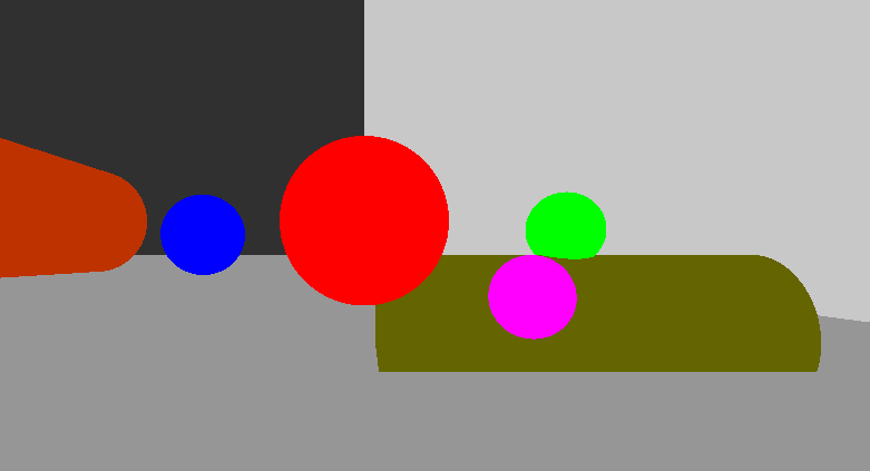
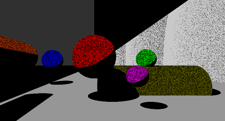
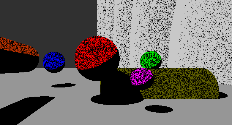
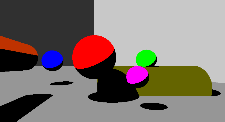
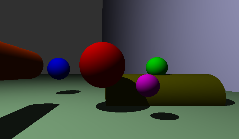
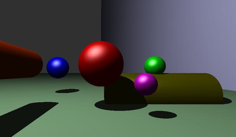
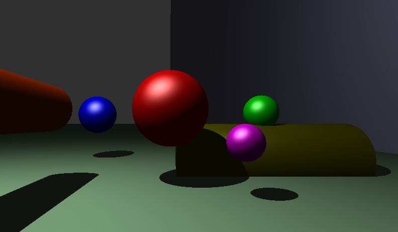
The same scene without any shadowing (a); shadowing without ensuring that the shadow ray-object intersection occurs in front of the light source (b); shadowing without offsetting the shadow ray origin, resulting in shadow acne (c), correct shadowing (d). Note that no shading has been applied yet and shadows are still rendered as black.

↥ back to top

---

Shading

Phong Reflection Model

As seen in the renders above, adding shadows helps enhance the sense of depth. However, the objects still appear relatively flat, as shadows alone don't fully account for how light interacts with surfaces.

To improve this, we can use the Phong Reflection Model, which simulates how light interacts with surfaces in three components:

1. Ambient Lighting: This represents the constant light that is scattered throughout the scene, illuminating all objects equally. It's the basic level of lighting that ensures no part of the object remains completely dark. Ambient light doesn’t depend on the object's position or orientation.

2. Diffuse Shading: This component simulates the light that hits a matte surface and scatters in many directions. The intensity of the diffuse reflection depends on the angle between the light source and the surface normal. The closer the light is to perpendicular, the brighter the object appears. This is what gives objects their color based on the light they receive (for example, a landscape under the direct noon sun appears bright, while the same landscape at sunset, with a more angled light, appears darker)

3. Specular Reflection: This represents the shiny, reflective highlights on smooth surfaces, like the glare from a polished metal or wet surface. Specular reflection is influenced by the angle between the light source, the surface normal, and the viewer’s perspective. The more directly aligned these angles are, the more intense the reflection. This is what creates the glossy or shiny look on objects.

Phong Reflection Model: Ambient Lighting + Diffuse Shading + Specular Reflection = Complete Shading Model.^[3]

Diffuse Shading

Lambert's Cosine Law explains how light reflects off rough or matte surfaces. It states that the amount of light reflected is proportional to the cosine of the angle between the surface normal and the light direction. This means that light striking a surface head-on is reflected most strongly, while light at an angle produces weaker reflections. This law is used to simulate how materials appear brighter when facing the light and darker at steeper angles.

The following function calculates the diffuse reflection coefficient, which is used to simulate how light interacts with matte surfaces.

/**
Calculates the diffuse reflection coefficient at an intersection point using Lambert's Cosine Law.
The diffuse coefficient determines how much light a surface receives based on the angle between the surface normal and the light source direction.
 
@param rt 		Pointer to the main structure.
@param ix 		Pointer to the intersection data.

@return		The diffuse lighting coefficient value [0.0, 1.0].
*/
static double	get_diffuse_coefficient(t_rt *rt, t_ix *ix)
{
	double	diffuse;            // Variable to store the diffuse lighting coefficient
	double	dot;                // Dot product of the surface normal and the light direction

	// Calculate the dot product between the surface normal and the light direction
	dot = vec3_dot(ix->normal, ix->light_dir);
	
	// If the dot product is negative, set it to zero (no diffuse reflection)
	if (dot < 0)
		dot = 0;
	
	// Apply the diffuse shading formula: dot product * light intensity * diffuse constant
	// 'K_DIFFUSE' controls the intensity of the diffuse shading [0.0, 1.0].
	diffuse = dot * rt->scene.light.ratio * K_DIFFUSE;

	return (diffuse);  // Return the diffuse lighting coefficient value [0.0, 1.0]
}

Specular Reflection

The following function calculates the specular reflection (or highlight) coefficient based on the Phong shading model. This component simulates the shiny appearance of a surface, contributing to the overall realism by adding reflections of light.

/**
Calculates the specular highlighting coefficient at an intersection point based on the Phong shading model.
The specular coefficient defines the intensity of the specular highlight, which contributes to the shiny appearance of a surface.

 @param rt 		Pointer to the main structure.
 @param ix 		Pointer to the intersection data.

 @return		The specular lighting coefficient value [0.0, 1.0].
*/
static double	get_specular_coefficient(t_rt *rt, t_ix *ix)
{
	double	specular;		// Variable to store the specular lighting coefficient
	double	dot;			// The dot product between the reflection vector and the view direction
	t_vec3	reflection_dir;		// The reflection direction vector
	t_vec3	view_dir;	 	// The view direction from the intersection to the camera

	// Calculate the reflection direction using the light direction and the surface normal
	reflection_dir = get_reflection(ix->light_dir, ix->normal);

  	// Calculate the view direction from the intersection point to the camera
	view_dir = vec3_sub(rt->scene.cam.pos, ix->hit_point);
	view_dir = vec3_norm(view_dir);

	// Calculate the dot product between the reflection direction and view direction
	dot = vec3_dot(reflection_dir, view_dir);

	// If the dot product is negative, set it to zero (no reflection)
	if (dot < 0)
		dot = 0;

	// Calculate the specular intensity using the Phong model: (dot^shininess) * light ratio * specular constant
	// 'K_SHININESS' controls the glossiness of the specular highlight (higher values result in a smaller, more focused highlight);
	// values between 3.0 and 10.0 are recommended.
	// 'K_SPECULAR' controls the intensity of the specular highlight [0.0, 1.0].
	specular = pow(dot, K_SHININESS) * rt->scene.light.ratio * K_SPECULAR;

	return (specular);
}

Combining Shading Components

The final shaded color for a pixel is calculated by combining the ambient, diffuse, and specular components for each RGB channel, with the result clamped to a maximum of 255 to prevent overflow. An additional light fading effect further enhances the realism of the render.

/**
Computes the shading for a pixel based on the object's color and light
properties.
 @param rt	Pointer to the main struct containing scene and light properties.
 @param ix	Pointer to the ray/pixel intersection data containing object and light information.

 @return	A `t_shade` struct with the computed shading components (ambient, diffuse, specular).
*/
t_shade	get_shading(t_rt *rt, t_ix *ix)
{
	t_shade	pix;

	// Set base color of the object from the intersection data
	pix.base = ix->hit_obj->color;

	// Set the light color from the scene light properties
	pix.light = rt->scene.light.color;

	// Set ambient color of the object (how it interacts with ambient light)
	pix.ambient = ix->hit_obj->color_in_amb;

	// Compute the diffuse reflection coefficient
	pix.diff_coeff = get_diffuse_coefficient(rt, ix);

	// Compute specular reflection coefficient
	pix.spec_coeff = get_specular_coefficient(rt, ix);

	// compute distance-based fade factor
	pix.fade = clamp(K_FADE * 100 / (ix->light_dist * ix->light_dist), 1.0);

	// Compute the diffuse component for each color channel (RGB)
	pix.diffuse.r = pix.base.r * pix.light.r / 255 * pix.diff_coeff * pix.fade;
	pix.diffuse.g = pix.base.g * pix.light.g / 255 * pix.diff_coeff * pix.fade;
	pix.diffuse.b = pix.base.b * pix.light.b / 255 * pix.diff_coeff * pix.fade;

	// Compute the specular component for each color channel (RGB)
	pix.specular.r = pix.light.r * pix.spec_coeff * pix.fade;
	pix.specular.g = pix.light.g * pix.spec_coeff * pix.fade;
	pix.specular.b = pix.light.b * pix.spec_coeff * pix.fade;

	// Compute the final shaded color by adding ambient, diffuse, and specular components
	// Clamp each color channel to a maximum of 255 to avoid overflow
	pix.shaded.r = clamp(pix.ambient.r + pix.diffuse.r + pix.specular.r, 255);
	pix.shaded.g = clamp(pix.ambient.g + pix.diffuse.g + pix.specular.g, 255);
	pix.shaded.b = clamp(pix.ambient.b + pix.diffuse.b + pix.specular.b, 255);

	return (pix);
}

(a)

(b)

(c)
The same scene with: ambient light and diffuse shading (a), specular highlighting (b), and light fading (c), resulting in a fully shaded render.

↥ back to top

---

Acknowledgements

• The incredible books Ray Tracing from the Ground Up by Kevin Suffern^[1] and The Ray Tracer Challenge by Jamis Buck^[3] are not only excellent and comprehensive resources on the subject, but also accessible guides to the concepts and mathematics behind ray tracing. Figures taken from these books are referenced accordingly.
• The project badge is from this repository by Ali Ogun.

References

[1] Suffern, K. (2007). Ray Tracing from the Ground Up. A K Peters.
[2] Buck, J. (2024). Perspective and Orthogonal Views. Available at: https://docs.dataminesoftware.com/StudioEM/Latest/VR_Help/Perpective%20and%20Orthogonal%20Modes.htm
[3] Datamine Software (2019). The Ray Tracer Challenge. The Pragmatic Programmers, LLC.