Port of Karpathy's micrograd
A tiny Autograd engine (with a bite! :)). Implements backpropagation (reverse-mode autodiff) over a dynamically built DAG and a small neural networks library on top of it with a PyTorch-like API. Both are tiny, with about 100 and 50 lines of code respectively. The DAG only operates over scalar values, so e.g. we chop up each neuron into all of its individual tiny adds and multiplies. However, this is enough to build up entire deep neural nets doing binary classification, as the demo notebook shows. Potentially useful for educational purposes.
Below is a slightly contrived example showing a number of possible supported operations:
use micrograd::engine::*;

let a = Value::new(-4.0);
let b = Value::new(2.0);
let mut c = a + b;
let mut d = a * b + b.pow(3.);
c = c + (c + 1.);
c = c + (1. + c + (-a));
d = d + (d * 2. + (b + a).relu());
d = d + (3. * d + (b - a).relu());
let e = c - d;
let f = e.pow(2.);
let mut g = f / 2.0;
g = g + (10.0 / f);
g.backward();
let (amg, bmg, gmg) = (a, b, g);

let tol = 1e-6;
// forward pass went well
assert_float_eq!(gmg.data(), 24.70408163265306, abs <= tol);
// backward pass went well
assert_float_eq!(amg.grad(), 138.83381924198252, abs <= tol);
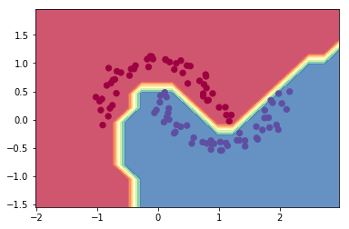
assert_float_eq!(bmg.grad(), 645.5772594752186, abs <= tol);The example demo.ipynb provides a full demo of training an 2-layer neural network (MLP) binary classifier. This is achieved by initializing a neural net from micrograd.nn module, implementing a simple svm "max-margin" binary classification loss and using SGD for optimization. As shown in the notebook, using a 2-layer neural net with two 16-node hidden layers we achieve the following decision boundary on the moon dataset:
For added convenience, the example complex_viz.rs produces graphviz visualizations. E.g. this one below is of a simple 2D neuron, arrived at by calling draw_dot on the code below, and it shows both the data (left number in each node) and the gradient (right number in each node).
extern crate micrograd;

use micrograd::engine::*;

fn main() {
    let a = Value::new(5.0);
    let b = 35.0 + a.pow(-3.) / -1.5;
    let c = b.relu();
    c.backward();

    let dot = viz::render_dot(c);
    println!("{dot}");
}

