This repository is for trigger-word detection/ digit recognition in speech using recurrent neural networks
Trigger word/ wake word detection is one of the most common applications of sequence models. The goal is to detect instances when a certain word is uttered, and more often than not, recognise the said word from amongst a small pool of "wake words"
In this repository, I demonstrate a GRU network, in combination with 1D Convolution, to detect three words:
One, Two and Three
The entire process has the following steps :
- Generate training dataset with labels.
- Convert audio files into spectrograms
- Train a combination of 1D Convolution and Recurrent layers to detect utterances.
All sounds in this project are taken from the Google speech commands dataset.
The dataset has 1 sec audio samples of a host of different words, but I will only be audio clips of the words "One", "Two" and "Three" and a combination of some other random words like "Bird", "Bed", "Happy", "House" which would be labelled as "negative"
The dataset also has various background noises, like "Someone doing the dishes", "Cat Meowing", "Running tap"
All these sounds will be combined in various proportions to generate 10 sec audio clips of words "One, Two and Three" superimposed over the background noises, along with the "negatives"
Concurrently, an array of labels will be generated, with each label being a one-hot encoded vector, like so:
[1.0, 0.0, 0.0, 0.0] => "One"
[0.0, 1.0, 0.0, 0.0] => "Two"
[0.0, 0.0, 1.0, 0.0] => "Three"
[0.0, 0.0, 0.0, 1.0] => "negative"
The 10 sec audio clips generated will be in ".wav" format. The WAV is a bitstream format. Loosely speaking, it contains time indexed chunks of silent and noisy patches to make up the audio file. Although the WAV file can be fed into a neural network as is, the network learns much better representations if spectrograms are used.
Any time varying signal can be broken down into its frequency components, by fourier decomposition, which is the idea that any signal can be expressed as the sum of sinusoids with different frequencies.
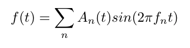
For any sound, spectral decomposition gives us the amplitudes of each of its frequency components. For example, a section of a violin being played can be broken down like so:

If such a decomposition is done at every time step of the audio signal and plotted, what results is a spectrogram.
For example, a harp clip taken from Chrome Music Lab: Spectrograms, looks like so:
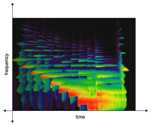
where the y-axis is the frequency and x-axis is time, and the colour represents the amplitude.
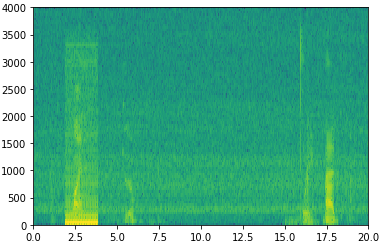
In our case, each audio clip is 10 sec long. In this program, I used pydub to input audio files, with a sampling rate of 200Hz, which means there will be 1 sample for every 5ms, making it about 2000 samples. If we plot the spectrogram of a sample training file ("train.wav" file in root directory), it looks like :
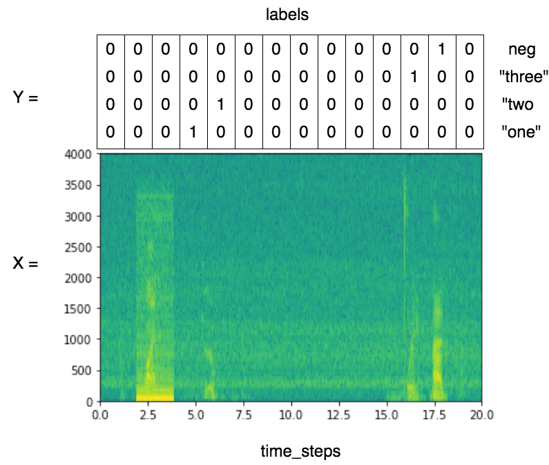
To train the model, we need to label the training data according to the utterances of the three words in the audio clips. Also, we want to detect time instances immediately after the words are uttered. To achieve this, the labelling process has the following steps :
- Get time segments where the target words (including negatives) are placed.
- Insert label vectors which have a length of 4 right after the segment ends
- Repeat the label for a fixed amount of time steps (in this program: 50). This is done to give the network some time to process the input before giving out the labels. A label which is only a single time step wide might not allow enough time for this.
For example, if you ignore the repeating of labels for illustration purposes, the training sample audio clip will be labelled as follows : (give it a listen)
A point to keep in mind is that the input time steps and output time steps might be different depending on the neural network architecture you use. Therefore, the output label time segments must be scaled accordingly.
All the methods used to generate the dataset are in the audio_data.py module. The entire dataset exists in the train_dir directory, along with test cases. The dataset consists of :
- 1000 indexed audio clips, 10 sec long, with various background sounds and negative words
- 1000 indexed labels in the form of a npy file, each label has the shape = (1375,4)
- 100 indexed audio clips, 10 sec long
- 100 indexed labels, each of shape (1375,4)
Note: You can easily generate more training and testing examples by setting the num_train and num_test variables in the audio_data.py file.
In this program, I used a combination of 1D convolution and GRUs, with intermittent dropout layers. It has two components, the input layer, which consists of:
- Input which has 1998 time steps, followed by..
- 1D Convolution layer, which shrinks the time steps to 1375
The 1375 time steps coming from the convolutional layer are then fed into a recurrent layer, which contains :
- Batch Normalization layer
- ReLu Activation layers
- Dropout layer with a dropout of 0.8
- GRU layer, with 128 hidden units
- Dropout(0.8)
- Batch Normalization
- GRY layer, with 128 hidden units
- Dropout(0.8)
- Batch Normalization
- Dropout(0.8)
- Dense layer with sigmoid activation as output.
Here is a detailed illustration of the model :
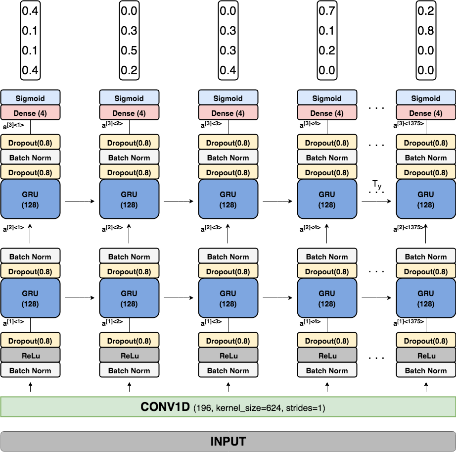
Note: the output values of the network are just for illustration purposes. This diagram was drawn using draw.io, its a cool tool and can be used to draw vector graphics.
tensor-flow summary of the model :
_________________________________________________________________
Layer (type)                 Output Shape              Param #
=================================================================
input_1 (InputLayer)         (None, 1998, 101)         0
_________________________________________________________________
conv1d_1 (Conv1D)            (None, 1375, 196)         12352900
_________________________________________________________________
batch_normalization_1 (Batch (None, 1375, 196)         784
_________________________________________________________________
activation_1 (Activation)    (None, 1375, 196)         0
_________________________________________________________________
dropout_1 (Dropout)          (None, 1375, 196)         0
_________________________________________________________________
gru_1 (GRU)                  (None, 1375, 128)         124800
_________________________________________________________________
dropout_2 (Dropout)          (None, 1375, 128)         0
_________________________________________________________________
batch_normalization_2 (Batch (None, 1375, 128)         512
_________________________________________________________________
gru_2 (GRU)                  (None, 1375, 128)         98688
_________________________________________________________________
dropout_3 (Dropout)          (None, 1375, 128)         0
_________________________________________________________________
batch_normalization_3 (Batch (None, 1375, 128)         512
_________________________________________________________________
dropout_4 (Dropout)          (None, 1375, 128)         0
_________________________________________________________________
time_distributed_1 (TimeDist (None, 1375, 4)           516
=================================================================
Total params: 12,578,712
Trainable params: 12,577,808
Non-trainable params: 904
_________________________________________________________________
Notice that there are a lot of Dropout layers. This is because the 1375 time steps that I am using to input in the recurrent layer is a considerably small representation-space, and the model tends to overfit really quickly without dropout. Usually the number of dropout operations is decided on a very trial and error based approach.
Finally, I used the Adam optimizer with custom parameters, with categorical_crossentropy as the loss function.
opt = Adam(lr=0.0001, beta_1=0.9, beta_2=0.999, decay=0.01)
model.compile(loss='categorical_crossentropy', optimizer=opt, metrics=["accuracy"])
After training it for 100 epochs, with a batch_size of 5, the model achieves an accuracy of 95%
Note: 95% does not mean anything in this case. Even if the model were to output all zeros, it would still count as about 90% accuracy because of the way the problem is set up.