Skip to content
New issue

Have a question about this project? Sign up for a free GitHub account to open an issue and contact its maintainers and the community.

By clicking “Sign up for GitHub”, you agree to our terms of service and privacy statement. We’ll occasionally send you account related emails.

Already on GitHub? Sign in to your account

2D time-dependent heat equation #61

Closed
wangcj05 opened this issue Jun 4, 2020 · 21 comments
Closed

2D time-dependent heat equation #61

wangcj05 opened this issue Jun 4, 2020 · 21 comments

Comments

@wangcj05
Copy link

wangcj05 commented Jun 4, 2020

Hello,

I tried to using DeepXDE to solve 2D time-dependent heat equations, i.e.
image

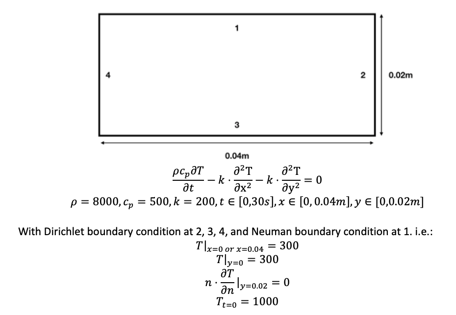
The following is my script:

import numpy as np
import tensorflow as tf
import matplotlib.pyplot as plt
import deepxde as dde
from scipy.interpolate import griddata
import matplotlib.gridspec as gridspec
from mpl_toolkits.mplot3d import axes3d

# geometry parameters
xdim = 200
ydim = 100
xmin = 0.0
ymin = 0.0
xmax = 0.04
ymax = 0.02
# input parameters

rho = 8000
cp = 500
k = 200
T0 = 1000

t0 = 0.0
te = 30.0
x_start = 0.0 # laser start position

# dnn parameters
num_hidden_layer = 3 # number of hidden layers for DNN
hidden_layer_size = 60 # size of each hidden layers
num_domain=1000 # number of training points within domain Tf: random points (spatio-temporal domain)
num_boundary=1000 # number of training boundary condition points on the geometry boundary: Tb
num_initial= 1000 # number of training initial condition points: Tb
num_test=None # number of testing points within domain: uniform generated
epochs=20000 # number of epochs for training
lr=0.001 # learning rate

def main():
    def pde(x, T):
        dT_x = tf.gradients(T, x)[0]
        dT_x, dT_y, dT_t = dT_x[:,0:1], dT_x[:,1:2], dT_x[:,2:]
        dT_xx = tf.gradients(dT_x, x)[0][:, 0:1]
        dT_yy = tf.gradients(dT_y, x)[0][:, 1:2]
        return rho*cp*dT_t -  k*dT_xx - k*dT_yy

    def boundary_x_l(x, on_boundary):
        return on_boundary and np.isclose(x[0], xmin)

    def boundary_x_r(x, on_boundary):
        return on_boundary and np.isclose(x[0], xmax)

    def boundary_y_b(x, on_boundary):
        return on_boundary and np.isclose(x[1], ymin)

    def boundary_y_u(x, on_boundary):
        return on_boundary and np.isclose(x[1], ymax)

    def func(x):
        return np.ones((len(x),1), dtype=np.float32)*T0

    def func_n(x):
        return np.zeros((len(x),1), dtype=np.float32)


    geom = dde.geometry.Rectangle([0, 0], [xmax, ymax])
    timedomain = dde.geometry.TimeDomain(t0, te)
    geomtime = dde.geometry.GeometryXTime(geom, timedomain)

    bc_x_l = dde.DirichletBC(geomtime, func, boundary_x_l)
    bc_x_r = dde.DirichletBC(geomtime, func, boundary_x_r)
    bc_y_b = dde.DirichletBC(geomtime, func, boundary_y_b)
    bc_y_u = dde.NeumannBC(geomtime, func_n, boundary_y_u)
    ic = dde.IC(geomtime, func, lambda _, on_initial: on_initial)

    data = dde.data.TimePDE(
        geomtime,
        pde,
        [bc_x_l, bc_x_r, bc_y_b, bc_y_u, ic],
        num_domain=num_domain,
        num_boundary=num_boundary,
        num_initial=num_initial,
        # train_distribution="uniform",
        num_test=num_test
    )
    net = dde.maps.FNN([3] + [hidden_layer_size] * num_hidden_layer + [1], "tanh", "Glorot uniform")
    model = dde.Model(data, net)

    model.compile("adam", lr=lr)
    losshistory, train_state = model.train(epochs=epochs)
    # model.compile("L-BFGS-B")
    # losshistory, train_state = model.train()
    dde.saveplot(losshistory, train_state, issave=False, isplot=False)

if __name__ == "__main__":
    main()

However, I could not get the converged solution. Basically, the errors on the boundary are not converging. See the following:

Step      Train loss                                                      Test loss                                                       Test metric
0         [1.62e+11, 1.00e+06, 1.00e+06, 1.00e+06, 6.38e-03, 1.00e+06]    [1.62e+11, 0.00e+00, 0.00e+00, 0.00e+00, 0.00e+00, 0.00e+00]    []
1000      [8.22e+05, 9.98e+05, 9.98e+05, 9.98e+05, 9.45e-04, 9.98e+05]    [8.22e+05, 0.00e+00, 0.00e+00, 0.00e+00, 0.00e+00, 0.00e+00]    []
2000      [8.14e+04, 9.96e+05, 9.96e+05, 9.96e+05, 9.77e-04, 9.96e+05]    [8.14e+04, 0.00e+00, 0.00e+00, 0.00e+00, 0.00e+00, 0.00e+00]    []
3000      [4.54e+04, 9.94e+05, 9.94e+05, 9.94e+05, 1.67e-03, 9.94e+05]    [4.54e+04, 0.00e+00, 0.00e+00, 0.00e+00, 0.00e+00, 0.00e+00]    []
4000      [3.79e+04, 9.92e+05, 9.92e+05, 9.92e+05, 1.74e-03, 9.92e+05]    [3.79e+04, 0.00e+00, 0.00e+00, 0.00e+00, 0.00e+00, 0.00e+00]    []
5000      [2.12e+04, 9.91e+05, 9.91e+05, 9.91e+05, 1.76e-03, 9.91e+05]    [2.12e+04, 0.00e+00, 0.00e+00, 0.00e+00, 0.00e+00, 0.00e+00]    []
6000      [1.20e+04, 9.89e+05, 9.89e+05, 9.89e+05, 1.45e-03, 9.89e+05]    [1.20e+04, 0.00e+00, 0.00e+00, 0.00e+00, 0.00e+00, 0.00e+00]    []

Do you have any suggestion how to fix this problem?

Thank you in advance!

@lululxvi
Copy link
Owner

lululxvi commented Jun 4, 2020

See "Q: I failed to train the network, e.g., the training loss is large." at "Questions & Answers" at the webpage.

Note: net.outputs_modify() is renamed to net.apply_output_transform()

@qizhang94
Copy link

I think you should normalize you PDE or apply network output transform, the scales of your parameters differ a lot.

@wangcj05
Copy link
Author

@lululxvi @qizhang94 Thanks a lot for your answers. I have tried to scale the problem. Since the solution for this problem is between [300, 1000]. I have rescaled the problem by 100. In addition, I have also tried to use the loss_weight to rescale the weight. However, the problem does not converge. Do you have any suggestions?

The updated code is provided:

mport numpy as np
import tensorflow as tf
import matplotlib.pyplot as plt
import deepxde as dde
from scipy.interpolate import griddata
import matplotlib.gridspec as gridspec
from mpl_toolkits.mplot3d import axes3d

# geometry parameters
xdim = 200
ydim = 100
xmin = 0.0
ymin = 0.0
xmax = 0.04
ymax = 0.02
# input parameters

rho = 8000
cp = 500
k = 200
T0 = 300
Tinit = 1000

t0 = 0.0
te = 30.0
x_start = 0.0 # laser start position

# dnn parameters
num_hidden_layer = 3 # number of hidden layers for DNN
hidden_layer_size = 40 # size of each hidden layers
num_domain=1000 # number of training points within domain Tf: random points (spatio-temporal domain)
num_boundary=1000 # number of training boundary condition points on the geometry boundary: Tb
num_initial= 1000 # number of training initial condition points: Tb
num_test=None # number of testing points within domain: uniform generated
epochs=10000 # number of epochs for training
lr=0.001 # learning rate

def main():
    def pde(x, T):
        dT_x = tf.gradients(T, x)[0]
        dT_x, dT_y, dT_t = dT_x[:,0:1], dT_x[:,1:2], dT_x[:,2:]
        dT_xx = tf.gradients(dT_x, x)[0][:, 0:1]
        dT_yy = tf.gradients(dT_y, x)[0][:, 1:2]
        return rho*cp*dT_t -  k*dT_xx - k*dT_yy

    def boundary_x_l(x, on_boundary):
        return on_boundary and np.isclose(x[0], xmin)

    def boundary_x_r(x, on_boundary):
        return on_boundary and np.isclose(x[0], xmax)

    def boundary_y_b(x, on_boundary):
        return on_boundary and np.isclose(x[1], ymin)

    def boundary_y_u(x, on_boundary):
        return on_boundary and np.isclose(x[1], ymax)

    def func(x):
        return np.ones((len(x),1), dtype=np.float32)*T0

    def func_n(x):
        return np.zeros((len(x),1), dtype=np.float32)

    def func_init(x):
        return np.ones((len(x),1), dtype=np.float32)*Tinit


    geom = dde.geometry.Rectangle([0, 0], [xmax, ymax])
    timedomain = dde.geometry.TimeDomain(t0, te)
    geomtime = dde.geometry.GeometryXTime(geom, timedomain)

    bc_x_l = dde.DirichletBC(geomtime, func, boundary_x_l)
    bc_x_r = dde.DirichletBC(geomtime, func, boundary_x_r)
    bc_y_b = dde.DirichletBC(geomtime, func, boundary_y_b)
    bc_y_u = dde.NeumannBC(geomtime, func_n, boundary_y_u)
    ic = dde.IC(geomtime, func_init, lambda _, on_initial: on_initial)

    data = dde.data.TimePDE(
        geomtime,
        pde,
        [bc_x_l, bc_x_r, bc_y_b, bc_y_u, ic],
        num_domain=num_domain,
        num_boundary=num_boundary,
        num_initial=num_initial,
        # train_distribution="uniform",
        num_test=num_test
    )
    net = dde.maps.FNN([3] + [hidden_layer_size] * num_hidden_layer + [1], "tanh", "Glorot uniform")
    # net.apply_output_transform(lambda x, y: y*1000)
    net.apply_output_transform(lambda x, y: y*100)
    model = dde.Model(data, net)

    model.compile("adam", lr=lr, loss_weights=[1e-12, 1e-2, 1e-2, 1e-2, 1, 1e-3])
    # model.compile("adam", lr=lr)
    losshistory, train_state = model.train(epochs=epochs)

    # model.compile("L-BFGS-B")
    # losshistory, train_state = model.train()
    dde.saveplot(losshistory, train_state, issave=False, isplot=False)

if __name__ == "__main__":
    main()

image

@lululxvi
Copy link
Owner

Try to train for more iterations.

@wangcj05
Copy link
Author

Try to train for more iterations.

@lululxvi, I have tried your suggestion, but the problem still does not converge (see the attached picture):

image

@lululxvi
Copy link
Owner

There are some problems of the scaling:

  1. Rescale the geometry, such that the domain is roughly [0, 1] x [0, 1]
  2. Try a small te first, e.g., 1
  3. The solution is of order 1000, not 100. I suggest to rescale the T, which is easy for your problem, instead of using net.apply_output_transform.

@wangcj05
Copy link
Author

@lululxvi I Thanks for your quick response. have tried different orders, i.e. 100 and 1000 using the net.apply_output_transform, the problem still suffers the convergence issue. I will try your suggestions to rescale the geometry and T with small end of time.

@Huzaifg
Copy link

Huzaifg commented Dec 8, 2021

Hello @wangcj05 ! I am trying to solve a similar problem. Did you achieve convergence?

@wangcj05
Copy link
Author

wangcj05 commented Dec 8, 2021

@Huzaifg Unfortunately, I do not get the problem converged.

@Huzaifg
Copy link

Huzaifg commented Jan 28, 2022

@wangcj05 I actually got this to work a while back but forgot to update here.
This is the equation I solved
Screenshot 2022-01-28 at 3 45 13 PM
First, I normalized the equation
Screenshot 2022-01-28 at 3 47 00 PM
And made some modifications to the boundary conditions
Screenshot 2022-01-28 at 3 48 30 PM
I also applied a output transform to ensure that the tempretures that the DNN was outputing were positive using
net.apply_output_transform(lambda x, y: abs(y))

Given below is the complete code

import deepxde as dde
import matplotlib.pyplot as plt
import numpy as np
from deepxde.backend import tf

# Some useful functions
t1 = 0
t2 = 1
end_time = 1

def pde(X,T):
    dT_xx = dde.grad.hessian(T, X ,j=0)
    dT_yy = dde.grad.hessian(T, X, j=1)
    dT_t = dde.grad.jacobian(T, X, j=2)
#     Dividing by rhoc to make it 1
    rhoc = (3.8151 * 10**3) / (3.8151 * 10**3)
    kap = (385 / (3.8151 * 10**3))
    # no forcing function
    return ((rhoc * dT_t) - (kap * (dT_xx + dT_yy)))


def r_boundary(X,on_boundary):
    x,y,t = X
    return on_boundary and np.isclose(x,1)
def l_boundary(X,on_boundary):
    x,y,t = X
    return on_boundary and np.isclose(x,0)
def up_boundary(X,on_boundary):
    x,y,t = X
    return on_boundary and np.isclose(y,1)
def down_boundary(X,on_boundary):
    x,y,t = X
    return on_boundary and np.isclose(y,0)

def boundary_initial(X, on_initial):
    x,y,t = X
    return on_initial and np.isclose(t, 0)

def init_func(X):
    x = X[:, 0:1]
    y = X[:, 1:2]
    t = np.zeros((len(X),1))
    for count,x_ in enumerate(x):
        if x_ < 0.5:
            t[count] = t1
        else:
            t[count] = t1 + (2) * (x_ - 0.5)
    return t
    
def dir_func_l(X):
    return t1 * np.ones((len(X),1))


def dir_func_r(X):
    return t2 * np.ones((len(X),1))

def func_zero(X):
    return np.zeros((len(X),1))
def hard(X, T):
    x,y,t = x[:, 0:1], x[:, 1:2],x[:,2:3]
    
    return (r - r_in) * y + T_star

num_domain = 30000
num_boundary = 8000
num_initial = 20000
layer_size = [3] + [60] * 5 + [1]
activation_func = "tanh"
initializer = "Glorot uniform"
lr = 1e-3
# Applying Loss weights as given below
# [PDE Loss, BC1 loss - Dirichlet Left , BC2 loss - Dirichlet Right, BC3 loss- Neumann up, BC4 loss - Neumann down, IC Loss]
loss_weights = [10, 1, 1, 1, 1, 10]
epochs = 10000
optimizer = "adam"
batch_size_ = 256

geom = dde.geometry.Rectangle(xmin=[0, 0], xmax=[1, 1])
timedomain = dde.geometry.TimeDomain(0, end_time)
geomtime = dde.geometry.GeometryXTime(geom, timedomain)

bc_l = dde.DirichletBC(geomtime, dir_func_l, l_boundary)
bc_r = dde.DirichletBC(geomtime, dir_func_r, r_boundary)
bc_up = dde.NeumannBC(geomtime, func_zero, up_boundary)
bc_low = dde.NeumannBC(geomtime, func_zero, down_boundary)
ic = dde.IC(geomtime, init_func, boundary_initial)


data = dde.data.TimePDE(
    geomtime, pde, [bc_l, bc_r, bc_up, bc_low, ic], num_domain=num_domain, num_boundary=num_boundary,  num_initial=num_initial)


net = dde.maps.FNN(layer_size, activation_func, initializer)
net.apply_output_transform(lambda x, y: abs(y))
## Uncomment below line to apply hard Dirichlet Boundary Conditions
# net.outputs_modify(lambda x, y: x[:,0:1]*t2 + x[:,0:1] * (1 - x[:,0:1]) * y)
model = dde.Model(data, net)

model.compile(optimizer, lr=lr,loss_weights=loss_weights)
# To save the best model every 1000 epochs
checker = dde.callbacks.ModelCheckpoint(
    "model/model1.ckpt", save_better_only=True, period=1000
)
losshistory, trainstate = model.train(epochs=epochs,batch_size = batch_size_,callbacks = [checker])
model.compile("L-BFGS-B")
dde.optimizers.set_LBFGS_options(
    maxcor=50,
)
losshistory, train_state = model.train(epochs = epochs, batch_size = batch_size_)
dde.saveplot(losshistory, trainstate, issave=True, isplot=True)

The best results achieved,
fiinal_comb
final_train
I also predicted the temperature for a paticular time frame using the code given below

import matplotlib.animation as animation
from matplotlib.animation import FuncAnimation


ax = fig.add_subplot(111)
nelx = 100
nely = 100
timesteps = 101
x = np.linspace(0,1,nelx+1)
y = np.linspace(0,1,nely+1)
t = np.linspace(0,1,timesteps)
delta_t = t[1] - t[0]
xx,yy = np.meshgrid(x,y)


x_ = np.zeros(shape = ((nelx+1) * (nely+1),))
y_ = np.zeros(shape = ((nelx+1) * (nely+1),))
for c1,ycor in enumerate(y):
    for c2,xcor in enumerate(x):
        x_[c1*(nelx+1) + c2] = xcor
        y_[c1*(nelx+1) + c2] = ycor
Ts = []
        
for time in t:
    t_ = np.ones((nelx+1) * (nely+1),) * (time)
    X = np.column_stack((x_,y_))
    X = np.column_stack((X,t_))
    T = model.predict(X)
    T = T*30
    T = T.reshape(T.shape[0],)
    T = T.reshape(nelx+1,nely+1)
    Ts.append(T)
def plotheatmap(T,time):
  # Clear the current plot figure
    plt.clf()
    plt.title(f"Temperature at t = {time*delta_t} unit time")
    plt.xlabel("x")
    plt.ylabel("y")
    plt.pcolor(xx, yy, T,cmap = 'RdBu_r')
    plt.colorbar()
    return plt

def animate(k):
    plotheatmap(Ts[k], k)
    
anim = animation.FuncAnimation(plt.figure(), animate, interval=1, frames=len(t), repeat=False)
    
anim.save("trial1.gif")

You can also find the gif converted to a mp4 file at the Gdrive link
https://drive.google.com/file/d/1t_uWzJT6ks1uMT0EKChcw7b-HqPJGtzW/view?usp=sharing

Please do let me know if I could have done something better or some mistakes that you find, I am only starting out and would love to learn!

@ADS-Astral
Copy link

@Huzaifg Thank you for an excellent explanation and code upload. Works perfectly.
Speaking as an IoT engineer this would have taken months to understand and problem solve.
has given a much deeper understanding of practical uses for deepXDE.

thanks again.

@Huzaifg
Copy link

Huzaifg commented Aug 29, 2022

Hey @MINE0126

Can you post your loss vs Epochs graph for the above result?

@MINE0126
Copy link

Hello, @Huzaifg
Thank you for your answer. I have solved this question.Thank again.
But I have a new problem #874.
Hope you can help me, thank you.

@WANGDI-1291
Copy link

Hi~ @MINE0126 Would you mind posting the correct code here? Thans in advance!

@123new-net
Copy link

@Huzaifg Hi.
I would like to know the parameters and region normalization about PDE. I see that the space-time regions in your model are all from 0 to 1, and divide rhoc and kap by 3.8E3. Is this related to the problem scaling described in the above discussion? I wanted to explore this aspect to see if it would help my model. Below are my PDE and space-time region codes. I hope you can give me some suggestions on normalization or scaling.

`a1=1.67e-4
a2=0.45
a3=5e-4
a4=0.45
def pde(x, u):
p,s = u[:, 0:1], u[:, 1:2]

dp_xx = dde.grad.hessian(u, x, component=0, i=0, j=0)
dp_yy = dde.grad.hessian(u, x, component=0, i=1, j=1)

ds_t = dde.grad.jacobian(u, x, i=1, j=2)

f_o=a1*(dp_xx+dp_yy)-a2*ds_t
f_w=a3*(dp_xx+dp_yy)+a4*ds_t

return [f_o,f_w]

geom = dde.geometry.Rectangle(xmin=[0,0], xmax=[5,5])
timedomain=dde.geometry.TimeDomain(0,30)
geomtime=dde.geometry.GeometryXTime(geom,timedomain)`

Thanks!

@Huzaifg
Copy link

Huzaifg commented Sep 1, 2022

Hello @123new-net ,
Yes, this was done to encounter the scaling problem as described above. I am unsure how you should go about scaling your problem, its been a while since I have solved a problem like this.

@WANGDI-1291
Copy link

Hi~ @Huzaifg The initial function needs to be 2 dimensional. But you just use "np.zeros((len(X),1))" here. So I'm wondering about this. Hope for your reply. Thanks!

@hannanmustajab
Copy link

Hey @Huzaifg, Your code above has been really helpful. Thank you for sharing with the community. I am quite new to DeepXDE, and have a few doubts. I was wondering if you might have any answers for them.

  1. When you define num_domain = 30000, how many points are actually created ? Is it 30000 in each space. So since we are having a 3D problem, it would be 30000*3 or it is 30000/3 ?
  2. I see you plotted the loss functions for each of the terms. Can you share your code snippets for that part ?

Hope for your reply.
Thanks
Hannan

@AJAXJR24
Copy link

AJAXJR24 commented Dec 8, 2023

  1. When you define num_domain = 30000, how many points are actually created ? Is it 30000 in each space. So since we are having a 3D problem, it would be 30000*3 or it is 30000/3 ?

Hi
None of the above. There will be 30000 points in your training. 30000 x and 30000 y and 30000 t. it's like:
[0,0.5,0], [0.1,0.5,0.3], .....

@Mouhamedsaw
Copy link

Hello everyone,

Does anyone have any experience with plotting the above solution $T$ versus time $t$, i.e. time (t) on the x-axis and temperature (T) on the y-axis.

Thank you in advance.

@Hari-IITian
Copy link

@wangcj05 I actually got this to work a while back but forgot to update here. This is the equation I solved Screenshot 2022-01-28 at 3 45 13 PM First, I normalized the equation Screenshot 2022-01-28 at 3 47 00 PM And made some modifications to the boundary conditions Screenshot 2022-01-28 at 3 48 30 PM I also applied a output transform to ensure that the tempretures that the DNN was outputing were positive using net.apply_output_transform(lambda x, y: abs(y))

Given below is the complete code

import deepxde as dde
import matplotlib.pyplot as plt
import numpy as np
from deepxde.backend import tf

# Some useful functions
t1 = 0
t2 = 1
end_time = 1

def pde(X,T):
    dT_xx = dde.grad.hessian(T, X ,j=0)
    dT_yy = dde.grad.hessian(T, X, j=1)
    dT_t = dde.grad.jacobian(T, X, j=2)
#     Dividing by rhoc to make it 1
    rhoc = (3.8151 * 10**3) / (3.8151 * 10**3)
    kap = (385 / (3.8151 * 10**3))
    # no forcing function
    return ((rhoc * dT_t) - (kap * (dT_xx + dT_yy)))


def r_boundary(X,on_boundary):
    x,y,t = X
    return on_boundary and np.isclose(x,1)
def l_boundary(X,on_boundary):
    x,y,t = X
    return on_boundary and np.isclose(x,0)
def up_boundary(X,on_boundary):
    x,y,t = X
    return on_boundary and np.isclose(y,1)
def down_boundary(X,on_boundary):
    x,y,t = X
    return on_boundary and np.isclose(y,0)

def boundary_initial(X, on_initial):
    x,y,t = X
    return on_initial and np.isclose(t, 0)

def init_func(X):
    x = X[:, 0:1]
    y = X[:, 1:2]
    t = np.zeros((len(X),1))
    for count,x_ in enumerate(x):
        if x_ < 0.5:
            t[count] = t1
        else:
            t[count] = t1 + (2) * (x_ - 0.5)
    return t
    
def dir_func_l(X):
    return t1 * np.ones((len(X),1))


def dir_func_r(X):
    return t2 * np.ones((len(X),1))

def func_zero(X):
    return np.zeros((len(X),1))
def hard(X, T):
    x,y,t = x[:, 0:1], x[:, 1:2],x[:,2:3]
    
    return (r - r_in) * y + T_star

num_domain = 30000
num_boundary = 8000
num_initial = 20000
layer_size = [3] + [60] * 5 + [1]
activation_func = "tanh"
initializer = "Glorot uniform"
lr = 1e-3
# Applying Loss weights as given below
# [PDE Loss, BC1 loss - Dirichlet Left , BC2 loss - Dirichlet Right, BC3 loss- Neumann up, BC4 loss - Neumann down, IC Loss]
loss_weights = [10, 1, 1, 1, 1, 10]
epochs = 10000
optimizer = "adam"
batch_size_ = 256

geom = dde.geometry.Rectangle(xmin=[0, 0], xmax=[1, 1])
timedomain = dde.geometry.TimeDomain(0, end_time)
geomtime = dde.geometry.GeometryXTime(geom, timedomain)

bc_l = dde.DirichletBC(geomtime, dir_func_l, l_boundary)
bc_r = dde.DirichletBC(geomtime, dir_func_r, r_boundary)
bc_up = dde.NeumannBC(geomtime, func_zero, up_boundary)
bc_low = dde.NeumannBC(geomtime, func_zero, down_boundary)
ic = dde.IC(geomtime, init_func, boundary_initial)


data = dde.data.TimePDE(
    geomtime, pde, [bc_l, bc_r, bc_up, bc_low, ic], num_domain=num_domain, num_boundary=num_boundary,  num_initial=num_initial)


net = dde.maps.FNN(layer_size, activation_func, initializer)
net.apply_output_transform(lambda x, y: abs(y))
## Uncomment below line to apply hard Dirichlet Boundary Conditions
# net.outputs_modify(lambda x, y: x[:,0:1]*t2 + x[:,0:1] * (1 - x[:,0:1]) * y)
model = dde.Model(data, net)

model.compile(optimizer, lr=lr,loss_weights=loss_weights)
# To save the best model every 1000 epochs
checker = dde.callbacks.ModelCheckpoint(
    "model/model1.ckpt", save_better_only=True, period=1000
)
losshistory, trainstate = model.train(epochs=epochs,batch_size = batch_size_,callbacks = [checker])
model.compile("L-BFGS-B")
dde.optimizers.set_LBFGS_options(
    maxcor=50,
)
losshistory, train_state = model.train(epochs = epochs, batch_size = batch_size_)
dde.saveplot(losshistory, trainstate, issave=True, isplot=True)

The best results achieved, fiinal_comb final_train I also predicted the temperature for a paticular time frame using the code given below

import matplotlib.animation as animation
from matplotlib.animation import FuncAnimation


ax = fig.add_subplot(111)
nelx = 100
nely = 100
timesteps = 101
x = np.linspace(0,1,nelx+1)
y = np.linspace(0,1,nely+1)
t = np.linspace(0,1,timesteps)
delta_t = t[1] - t[0]
xx,yy = np.meshgrid(x,y)


x_ = np.zeros(shape = ((nelx+1) * (nely+1),))
y_ = np.zeros(shape = ((nelx+1) * (nely+1),))
for c1,ycor in enumerate(y):
    for c2,xcor in enumerate(x):
        x_[c1*(nelx+1) + c2] = xcor
        y_[c1*(nelx+1) + c2] = ycor
Ts = []
        
for time in t:
    t_ = np.ones((nelx+1) * (nely+1),) * (time)
    X = np.column_stack((x_,y_))
    X = np.column_stack((X,t_))
    T = model.predict(X)
    T = T*30
    T = T.reshape(T.shape[0],)
    T = T.reshape(nelx+1,nely+1)
    Ts.append(T)
def plotheatmap(T,time):
  # Clear the current plot figure
    plt.clf()
    plt.title(f"Temperature at t = {time*delta_t} unit time")
    plt.xlabel("x")
    plt.ylabel("y")
    plt.pcolor(xx, yy, T,cmap = 'RdBu_r')
    plt.colorbar()
    return plt

def animate(k):
    plotheatmap(Ts[k], k)
    
anim = animation.FuncAnimation(plt.figure(), animate, interval=1, frames=len(t), repeat=False)
    
anim.save("trial1.gif")

You can also find the gif converted to a mp4 file at the Gdrive link https://drive.google.com/file/d/1t_uWzJT6ks1uMT0EKChcw7b-HqPJGtzW/view?usp=sharing

Please do let me know if I could have done something better or some mistakes that you find, I am only starting out and would love to learn!

here if we reduce num_initial points to 400. then we get absurd result. so can you tell the approach to solve 2d heat equation with less initial points

Sign up for free to join this conversation on GitHub. Already have an account? Sign in to comment
Labels
None yet
Projects
None yet
Development

No branches or pull requests