-
-
Notifications
You must be signed in to change notification settings - Fork 48
/
Copy pathdocs.json
1 lines (1 loc) · 148 KB
/
docs.json
1
[{"name":"Axis","comment":" The axis component renders human-readable reference marks for scales. This\nalleviates one of the more tedious tasks in visualizing data.\n\nRenders an Axis based on a [Scale](./Scale).\n\n view =\n svg []\n [ g [ class [ \"axis\" ], transform [ Translate 0 300 ] ]\n [ Axis.left [ tickCount 10] myScale\n ]\n [\n\nRegardless of orientation, axes are always rendered at the origin. To change the\nposition of the axis with respect to the chart, specify a transform attribute on\nthe containing element.\n\n@docs RenderableScale, left, right, bottom, top\n\n\n### Customizing the axis\n\nThe elements created by the axis are considered part of its public API.\nYou can apply external stylesheets to\ncustomize the axis appearance. An axis consists of a path element of class\n“domain” representing the extent of the scale’s domain, followed by transformed\n`g` elements of class “tick” representing each of the scale’s ticks. Each tick has\na `line` element to draw the tick line, and a `text` element for the tick label.\nFor example, here is a typical bottom-oriented axis:\n\n <g fill=\"none\" font-size=\"10\" font-family=\"sans-serif\" text-anchor=\"middle\">\n <path class=\"domain\" stroke=\"#000\" d=\"M0.5,6V0.5H880.5V6\"></path>\n <g class=\"tick\" opacity=\"1\" transform=\"translate(0,0)\">\n <line stroke=\"#000\" y2=\"6\" x1=\"0.5\" x2=\"0.5\"></line>\n <text fill=\"#000\" y=\"9\" x=\"0.5\" dy=\"0.71em\">0.0</text>\n </g>\n <g class=\"tick\" opacity=\"1\" transform=\"translate(176,0)\">\n <line stroke=\"#000\" y2=\"6\" x1=\"0.5\" x2=\"0.5\"></line>\n <text fill=\"#000\" y=\"9\" x=\"0.5\" dy=\"0.71em\">0.2</text>\n </g>\n <g class=\"tick\" opacity=\"1\" transform=\"translate(352,0)\">\n <line stroke=\"#000\" y2=\"6\" x1=\"0.5\" x2=\"0.5\"></line>\n <text fill=\"#000\" y=\"9\" x=\"0.5\" dy=\"0.71em\">0.4</text>\n </g>\n <g class=\"tick\" opacity=\"1\" transform=\"translate(528,0)\">\n <line stroke=\"#000\" y2=\"6\" x1=\"0.5\" x2=\"0.5\"></line>\n <text fill=\"#000\" y=\"9\" x=\"0.5\" dy=\"0.71em\">0.6</text>\n </g>\n <g class=\"tick\" opacity=\"1\" transform=\"translate(704,0)\">\n <line stroke=\"#000\" y2=\"6\" x1=\"0.5\" x2=\"0.5\"></line>\n <text fill=\"#000\" y=\"9\" x=\"0.5\" dy=\"0.71em\">0.8</text>\n </g>\n <g class=\"tick\" opacity=\"1\" transform=\"translate(880,0)\">\n <line stroke=\"#000\" y2=\"6\" x1=\"0.5\" x2=\"0.5\"></line>\n <text fill=\"#000\" y=\"9\" x=\"0.5\" dy=\"0.71em\">1.0</text>\n </g>\n </g>\n\n@docs Attribute, ticks, tickFormat, tickCount, tickSizeInner, tickSizeOuter, tickPadding\n\n","unions":[{"name":"Attribute","comment":" ","args":["data"],"cases":[]}],"aliases":[{"name":"RenderableScale","comment":" Axes are rendered based on a [`Scale`](./Scale).\n\nCurrently only continuous (including time), quantize and band (via the `toRenderable` function) scales are supported.\n\n","args":["a","domain","range","value"],"type":"Scale.Scale { a | ticks : domain -> Basics.Int -> List.List value, domain : domain, tickFormat : domain -> Basics.Int -> value -> String.String, convert : domain -> range -> value -> Basics.Float, range : range, rangeExtent : domain -> range -> ( Basics.Float, Basics.Float ) }"}],"values":[{"name":"bottom","comment":" A bottom oriented axis. In this orientation, ticks are drawn below the horizontal domain path.\n","type":"List.List (Axis.Attribute value) -> Axis.RenderableScale a domain range value -> Svg.Svg msg"},{"name":"left","comment":" A left oriented axis. In this orientation, ticks are drawn to the left of the vertical domain path.\n","type":"List.List (Axis.Attribute value) -> Axis.RenderableScale a domain range value -> Svg.Svg msg"},{"name":"right","comment":" A right oriented axis. In this orientation, ticks are drawn to the right of the vertical domain path.\n","type":"List.List (Axis.Attribute value) -> Axis.RenderableScale a domain range value -> Svg.Svg msg"},{"name":"tickCount","comment":" How many tickmarks to approximately generate. Defaults to 10.\n","type":"Basics.Int -> Axis.Attribute data"},{"name":"tickFormat","comment":" A formatting function for the tick marks. Defaults to `Scale.tickFormat`.\n","type":"(data -> String.String) -> Axis.Attribute data"},{"name":"tickPadding","comment":" Padding controls the space between tick marks and tick labels. Defaults to 3.\n","type":"Basics.Float -> Axis.Attribute data"},{"name":"tickSizeInner","comment":" The inner tick size controls the length of the tick lines, offset from the native position of the axis.\nDefaults to 6.\n","type":"Basics.Float -> Axis.Attribute data"},{"name":"tickSizeOuter","comment":" The outer tick size controls the length of the square ends of the domain path, offset from the native position of the axis. Thus, the “outer ticks” are not actually ticks but part of the domain path, and their position is determined by the associated scale’s domain extent. Thus, outer ticks may overlap with the first or last inner tick. An outer tick size of 0 suppresses the square ends of the domain path, instead producing a straight line. Defaults to 6.\n","type":"Basics.Float -> Axis.Attribute data"},{"name":"ticks","comment":" Pass a list of ticks to be rendered explicitely. Defaults to `Scale.ticks`.\nUseful when you want to render the data points as ticks.\n","type":"List.List data -> Axis.Attribute data"},{"name":"top","comment":" A top oriented axis. In this orientation, ticks are drawn above the horizontal domain path.\n","type":"List.List (Axis.Attribute value) -> Axis.RenderableScale a domain range value -> Svg.Svg msg"}],"binops":[]},{"name":"Brush","comment":" Brushing is the interactive specification of a one- or two-dimensional selected region using a pointing gesture, such as by clicking and dragging the mouse. Brushing is often used to select discrete elements, such as dots in a scatterplot or files on a desktop. It can also be used to zoom-in to a region of interest, or to select continuous regions for cross-filtering data.\n\nThis module implements brushing for mouse events using SVG. Click and drag on the brush selection to translate the selection. Click and drag on one of the selection handles to move the corresponding edge (or edges) of the selection. Click and drag on the invisible overlay to define a new brush selection, or click anywhere within the brushable region while holding down the META (⌘) key. Holding down the ALT (⌥) key while moving the brush causes it to reposition around its center. Holding SHIFT (⇧) locks the dragging to a single dimension.\n\n@docs Brush, OneDimensional, TwoDimensional\n\n\n## Configuring the Brush behavior\n\nInitializing the brush always requires you to specify in local coordinates the rectangular region where the brush will be active.\n\n@docs initX, initY, initXY, Extent, keyboardModifiersEnabled\n\n\n## Querying the brush state\n\n@docs selection1d, selection2d\n\n\n## Updating the Brush\n\n@docs OnBrush, update, subscriptions\n\n\n## Manipulating the Selection\n\n@docs setSelection1d, setSelection2d, clearSelection, TransitionOption, instantly\n\n\n## View\n\n@docs view, Attribute, selectedArea, handleSize\n\nThe handle customization functions take a suggested extent for where you should draw them.\nThis is basically the line/point they represent extended by `handleSize / 2` in each direction.\nHowever, you do not need to abide by these dimensions exactly, you can render much larger or smaller objects there.\n\n@docs bottomHandle, leftHandle, rightHandle, topHandle, topLeftHandle, topRightHandle, bottomLeftHandle, bottomRightHandle\n\n","unions":[{"name":"Attribute","comment":" This is a type used to customize the view function of this module. However most of the functions that produce the type\nmay appear to also consume it. However, this is not the case, the functions take VirtualDom attributes, but produce this Attribute type.\n","args":["msg"],"cases":[]},{"name":"Brush","comment":" Encapsulates all the data we need to maintain the state of the brush. The dimension type variable can either be `OneDimensional` or `TwoDimensional`. This allows us to share a lot of the implementation details as well as implement generic UI customizations over brushes regardless of their dimensionality.\n\nYou will typically want to store this in your model.\n\n","args":["dimension"],"cases":[]},{"name":"OnBrush","comment":" This is the Msg type that this module uses for communicating between the update and the view.\n\nNote that when handling these messages, it is also extremely likely that the brush selection has somehow changed, so you can also use that place in your update function to react to that.\n\n","args":[],"cases":[]},{"name":"OneDimensional","comment":" ","args":[],"cases":[]},{"name":"TransitionOption","comment":" ","args":[],"cases":[]},{"name":"TwoDimensional","comment":" ","args":[],"cases":[]}],"aliases":[{"name":"Extent","comment":" Defines a rectangular region.\n","args":[],"type":"{ top : Basics.Float, bottom : Basics.Float, left : Basics.Float, right : Basics.Float }"}],"values":[{"name":"bottomHandle","comment":" Customise how to render the bottom handle.\n","type":"(Brush.Extent -> List.List (Svg.Attribute msg) -> Svg.Svg msg) -> Brush.Attribute msg"},{"name":"bottomLeftHandle","comment":" Customise how to render the bottom left handle. Only applies to a 2D brush.\n","type":"(Brush.Extent -> List.List (Svg.Attribute msg) -> Svg.Svg msg) -> Brush.Attribute msg"},{"name":"bottomRightHandle","comment":" Customise how to render the bottom right handle. Only applies to a 2D brush.\n","type":"(Brush.Extent -> List.List (Svg.Attribute msg) -> Svg.Svg msg) -> Brush.Attribute msg"},{"name":"clearSelection","comment":" Clears the selection programmatically.\n\n brush\n |> Brush.clearSelection\n |> Brush.selection1d --> Nothing\n\n","type":"Brush.Brush dim -> Brush.Brush dim"},{"name":"handleSize","comment":" The number in pixels which determines the size of the handles.\n","type":"Basics.Float -> Brush.Attribute msg"},{"name":"initX","comment":" Initializes a brush that allows brushing in the X axis.\n","type":"Brush.Extent -> Brush.Brush Brush.OneDimensional"},{"name":"initXY","comment":" Initializes a two dimensional brush.\n","type":"Brush.Extent -> Brush.Brush Brush.TwoDimensional"},{"name":"initY","comment":" Initializes a brush that allows brushing in the Y axis.\n","type":"Brush.Extent -> Brush.Brush Brush.OneDimensional"},{"name":"instantly","comment":" Perfom the update to the brush instantly, rather than with an animation (animations are not supported yet.)\n","type":"Brush.TransitionOption"},{"name":"keyboardModifiersEnabled","comment":" By default the brush will use the meta/alt and shift keys to change behavior. You can disable this with this function.\n","type":"Basics.Bool -> Brush.Brush dimension -> Brush.Brush dimension"},{"name":"leftHandle","comment":" Customise how to render the left handle.\n","type":"(Brush.Extent -> List.List (Svg.Attribute msg) -> Svg.Svg msg) -> Brush.Attribute msg"},{"name":"rightHandle","comment":" Customise how to render the right handle.\n","type":"(Brush.Extent -> List.List (Svg.Attribute msg) -> Svg.Svg msg) -> Brush.Attribute msg"},{"name":"selectedArea","comment":" Customize rendering for the rectangular region that is the selection.\n\nThe first argument is the actual coordinates of the selection, the second are the event handlers.\n\nThe default version renderes a `<rect fill=\"#777\" fill-opacity=\"0.3\" stroke=\"white\" shape-rendering=\"crispEdges\">`.\n\n","type":"(Brush.Extent -> List.List (Svg.Attribute msg) -> Svg.Svg msg) -> Brush.Attribute msg"},{"name":"selection1d","comment":" Exposes the selection for a single dimensional brush, where the first number should always be less than the second.\n","type":"Brush.Brush Brush.OneDimensional -> Maybe.Maybe ( Basics.Float, Basics.Float )"},{"name":"selection2d","comment":" Exposes the selection for a two dimensional brush.\n","type":"Brush.Brush Brush.TwoDimensional -> Maybe.Maybe Brush.Extent"},{"name":"setSelection1d","comment":" Programatically set the selection of the Brush.\n","type":"Brush.TransitionOption -> ( Basics.Float, Basics.Float ) -> Brush.Brush Brush.OneDimensional -> Brush.Brush Brush.OneDimensional"},{"name":"setSelection2d","comment":" Programatically set the selection of the Brush (in two dimensions).\n","type":"Brush.TransitionOption -> Brush.Extent -> Brush.Brush Brush.TwoDimensional -> Brush.Brush Brush.TwoDimensional"},{"name":"subscriptions","comment":" Don't forget the subscriptions, otherwise drag gestures won't work!\n","type":"Brush.Brush dim -> (Brush.OnBrush -> msg) -> Platform.Sub.Sub msg"},{"name":"topHandle","comment":" Customise how to render the top handle.\n","type":"(Brush.Extent -> List.List (Svg.Attribute msg) -> Svg.Svg msg) -> Brush.Attribute msg"},{"name":"topLeftHandle","comment":" Customise how to render the top left handle. Only applies to a 2D brush.\n","type":"(Brush.Extent -> List.List (Svg.Attribute msg) -> Svg.Svg msg) -> Brush.Attribute msg"},{"name":"topRightHandle","comment":" Customise how to render the top right handle. Only applies to a 2D brush.\n","type":"(Brush.Extent -> List.List (Svg.Attribute msg) -> Svg.Svg msg) -> Brush.Attribute msg"},{"name":"update","comment":" Call this in your update function to make the brush work!\n","type":"Brush.OnBrush -> Brush.Brush dim -> Brush.Brush dim"},{"name":"view","comment":" Actually renders the the brush selection widget. You can customise the appearance by passing in functions to render the individual pieces.\n\nThe actual widget consists of:\n\n1. An overlay invisible rectange which covers the interactive area.\n2. The selection rectangle.\n3. Handles in each direction the brush supports being dragged to.\n\n","type":"List.List (Brush.Attribute msg) -> (Brush.OnBrush -> msg) -> Brush.Brush dim -> Svg.Svg msg"}],"binops":[]},{"name":"Force","comment":" This module implements a velocity Verlet numerical integrator for simulating physical forces on particles.\nThe simulation is simplified: it assumes a constant unit time step _Δt = 1_ for each step, and a constant unit\nmass _m = 1_ for all particles. As a result, a force _F_ acting on a particle is equivalent to a constant\nacceleration _a_ over the time interval _Δt_, and can be simulated simply by adding to the particle’s velocity,\nwhich is then added to the particle’s position.\n\n[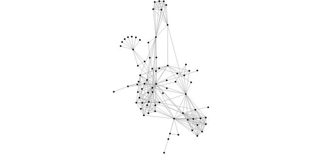](https://elm-visualization.netlify.app/ForceDirectedGraph/)\n\nIn the domain of information visualization, physical simulations are useful for studying networks and hierarchies!\n\n\n## Simulation\n\n@docs Entity, entity, simulation, State, isCompleted, reheat, iterations, computeSimulation, tick\n\n\n## Forces\n\n@docs Force, center, links, customLinks, manyBody, manyBodyStrength, customManyBody, collision, customCollision\n\nThe x- and y-positioning forces push nodes towards a desired position along the given dimension with a configurable strength. The strength of the force is proportional to the one-dimensional distance between the node’s position and the target position.\n\n@docs towardsX, towardsY, customRadial\n\n","unions":[{"name":"Force","comment":" A force modifies nodes’ positions or velocities; in this context, a force can apply a classical physical force such\nas electrical charge or gravity, or it can resolve a geometric constraint, such as keeping nodes within a bounding box\nor keeping linked nodes a fixed distance apart.\n","args":["comparable"],"cases":[]},{"name":"State","comment":" This holds internal state of the simulation.\n","args":["comparable"],"cases":[]}],"aliases":[{"name":"Entity","comment":" Force needs to compute and update positions and velocities on any objects that it is simulating.\nHowever, you can use your own data structure to manage these, as long as the individual objects expose the necessary\nproperties. Therefore this type alias is an extensible record allowing you to avoid excessive nesting.\n\nThe `id` property must be unique among objects, otherwise some of the colliding objects will be ignored by the simulation.\n\nAlso take care when initializing the positions so that the points don't overlap.\n\n","args":["comparable","a"],"type":"{ a | x : Basics.Float, y : Basics.Float, vx : Basics.Float, vy : Basics.Float, id : comparable }"}],"values":[{"name":"center","comment":" The centering force translates nodes uniformly so that the mean position of all nodes (the center of mass) is at\nthe given position ⟨x,y⟩. This force modifies the positions of nodes on each application; it does not modify velocities,\nas doing so would typically cause the nodes to overshoot and oscillate around the desired center. This force helps keep\nnodes in the center of the viewport, and it does not distort their relative positions.\n","type":"Basics.Float -> Basics.Float -> Force.Force comparable"},{"name":"collision","comment":" The collision force simulates each node as a circle with a given radius and modifies their velocities to prevent the circles from overlapping.\n\nPass in the radius and a list of nodes that you would like the force to apply to.\n\n","type":"Basics.Float -> List.List comparable -> Force.Force comparable"},{"name":"computeSimulation","comment":" This will run the entire simulation until it is completed and then returns the entities. Essentially keeps calling\n`tick` until the simulation is done.\n\nNote that this is fairly computationally expensive and may freeze the UI for a while if the dataset is large.\n\n","type":"Force.State comparable -> List.List (Force.Entity comparable a) -> List.List (Force.Entity comparable a)"},{"name":"customCollision","comment":" This allows you to specify a radius for each node specifically.\n\n**Strength:** Overlapping nodes are resolved through iterative relaxation. For each node, the other nodes that are anticipated to overlap at the next tick (using the anticipated positions ⟨x + vx,y + vy⟩) are determined; the node’s velocity is then modified to push the node out of each overlapping node. The change in velocity is dampened by the force’s strength such that the resolution of simultaneous overlaps can be blended together to find a stable solution. Set it to a value [0, 1], `collision` defaults to 1.\n\n**Iterations:** `collision` defaults to 1 - this makes the constraint more rigid, but makes the computation slower.\n\n","type":"{ iterations : Basics.Int, strength : Basics.Float } -> List.List ( comparable, Basics.Float ) -> Force.Force comparable"},{"name":"customLinks","comment":" Allows you to specify the link distance and optionally the strength. You must also specify the iterations count (the default in `links` is 1). Increasing the number of iterations greatly increases the rigidity of the constraint and is useful for complex structures such as lattices, but also increases the runtime cost to evaluate the force.\n","type":"Basics.Int -> List.List { source : comparable, target : comparable, distance : Basics.Float, strength : Maybe.Maybe Basics.Float } -> Force.Force comparable"},{"name":"customManyBody","comment":" This is the most flexible, but complex way to specify many body forces.\n\nThe first argument, let's call it _theta_, controls how much approximation to apply. The default value is 0.9.\n\nTo accelerate computation, this force implements the [Barnes–Hut approximation](http://en.wikipedia.org/wiki/Barnes%E2%80%93Hut_simulation) which takes O(n log n) per application where n is the number of nodes. For each application, a quadtree stores the current node positions; then for each node, the combined force of all other nodes on the given node is computed. For a cluster of nodes that is far away, the charge force can be approximated by treating the cluster as a single, larger node. The theta parameter determines the accuracy of the approximation: if the ratio w / l of the width w of the quadtree cell to the distance l from the node to the cell’s center of mass is less than theta, all nodes in the given cell are treated as a single node rather than individually. Setting this to 0 will disable the optimization.\n\nThis function also allows you to set the force strength individually on each node.\n\n","type":"Basics.Float -> List.List ( comparable, Basics.Float ) -> Force.Force comparable"},{"name":"customRadial","comment":" A positioning force that pushes towards the nearest point on the given circle.\n","type":"List.List ( comparable, { strength : Basics.Float, x : Basics.Float, y : Basics.Float, radius : Basics.Float } ) -> Force.Force comparable"},{"name":"entity","comment":" This is a convenience function for wrapping data up as Entities. The initial position of entities is arranged\nin a [phylotaxic pattern](https://elm-visualization.netlify.app/Petals/). Goes well with `List.indexedMap`.\n","type":"Basics.Int -> a -> Force.Entity Basics.Int { value : a }"},{"name":"isCompleted","comment":" Has the simulation stopped?\n","type":"Force.State comparable -> Basics.Bool"},{"name":"iterations","comment":" You can set this to control how quickly the simulation should converge. The default value is 300 iterations.\n\nLower number of iterations will produce a layout quicker, but risk getting stuck in a local minimum. Higher values take\nlonger, but typically produce better results.\n\n","type":"Basics.Int -> Force.State comparable -> Force.State comparable"},{"name":"links","comment":" The link force pushes linked nodes together or apart according to the desired link distance. The strength of the\nforce is proportional to the difference between the linked nodes’ distance and the target distance, similar to a spring\nforce.\n\nThe link distance here is 30, the strength of the force is proportional to the number of links on each side of the\npresent link, according to the formule: `1 / min (count souce) (count target)` where `count` if a function that counts\nlinks connected to those nodes.\n\n","type":"List.List ( comparable, comparable ) -> Force.Force comparable"},{"name":"manyBody","comment":" The many-body (or n-body) force applies mutually amongst all nodes. It can be used to simulate gravity (attraction)\nif the strength is positive, or electrostatic charge (repulsion) if the strength is negative.\n\nUnlike links, which only affect two linked nodes, the charge force is global: it affects all nodes whose ids are passed\nto it.\n\nThe default strength is -30 simulating a repulsing charge.\n\n","type":"List.List comparable -> Force.Force comparable"},{"name":"manyBodyStrength","comment":" This allows you to specify the strength of the many-body force.\n","type":"Basics.Float -> List.List comparable -> Force.Force comparable"},{"name":"reheat","comment":" Resets the computation. This is useful if you need to change the parameters at runtime, such as the position or\nvelocity of nodes during a drag operation.\n","type":"Force.State comparable -> Force.State comparable"},{"name":"simulation","comment":" Create a new simulation by passing a list of forces.\n","type":"List.List (Force.Force comparable) -> Force.State comparable"},{"name":"tick","comment":" Advances the simulation a single tick, returning both updated entities and a new State of the simulation.\n","type":"Force.State comparable -> List.List (Force.Entity comparable a) -> ( Force.State comparable, List.List (Force.Entity comparable a) )"},{"name":"towardsX","comment":" A positioning force along the X axis.\n","type":"List.List { node : comparable, strength : Basics.Float, target : Basics.Float } -> Force.Force comparable"},{"name":"towardsY","comment":" A positioning force along the Y axis.\n","type":"List.List { node : comparable, strength : Basics.Float, target : Basics.Float } -> Force.Force comparable"}],"binops":[]},{"name":"Hierarchy","comment":" Hierarchical data has its own visualization requirements, since usually the parent-child relationships\ntend to be important in understanding the dataset.\n\nThis module implements several layout techniques for visualizing such data.\n\n\n## Basic types\n\n\n### `Tree a`\n\nThe tree type used here comes from the gampleman/elm-rosetree package, which is a fully featured and performant\nlibrary fro dealing with trees. It has several methods you can use to convert other datastructures you may have\ninto that format and use it for visualizing your data.\n\n@docs Attribute, Supported, none\n\n\n### Return types\n\nMost of the layouts return a record with `x`, `y`, `width` and `height` attributes. Naturally the simplest is\nto take these values literally and simply produce a rectangle with these properties. However, these can be\nprofitably interpreted abstractly. For instance one may produce a horizontal diagram by simply switching `x` with\n`y` and `width` with `height`. Or treat `x` and `x + width` as angles in a radial layout.\n\n\n# Layouts\n\n@docs tidy, partition, treemap\n\n\n# Options\n\n@docs size, nodeSize, layered, parentChildMargin, peerMargin, padding, paddingOuter, paddingInner, paddingTop, paddingBottom, paddingLeft, paddingRight, tile\n\n\n## Tiling methods\n\n@docs slice, dice, sliceDice, squarify, squarifyRatio, TilingMethod\n\n","unions":[{"name":"Attribute","comment":" Each of the layout functions can be customized using a number of optional\narguments; these are represented by this type.\n\nThe first type argument represents the data contained in your tree, the second\nis a phantom type that ensures only valid options are passed to each layout\nmethod.\n\n","args":["a","attr"],"cases":[]},{"name":"Supported","comment":" Used to indicate which attributes go with which layout functions.\n\nFor instance, `padding` returns :\n\n Attribute a { b | padding = Supported }\n\nnow `partition` takes as its first argument:\n\n List (Attribute a { padding = Supported, size = Supported })\n\nThe compiler is quite happy to unify these types, but for instance\npassing this to `tidy` would cause a type error. It also makes it quite\neasy to understand from the type signature which options are supported.\n\n","args":[],"cases":[]}],"aliases":[{"name":"TilingMethod","comment":" You can implement your own tiling method as it's just a function. It recieves the following arguments:\n\n - depth: how many ancestors does the current node have\n - the bounding box of the current node\n - the quantitative value of the current node\n - the values of all the children nodes\n\nIt is expected to return the bounding boxes of the children.\n\nFor example, slice can be implemented like this (slightly simplified):\n\n slice : TilingMethod\n slice _ { x0, x1, y0, y1 } value children =\n List.foldl\n (\\childValue ( prevY, lst ) ->\n let\n nextY =\n prevY + childValue * ((y1 - y0) / value)\n in\n ( nextY, { x0 = x0, x1 = x1, y0 = prevY, y1 = nextY } :: lst )\n )\n ( y0, [] )\n children\n |> Tuple.second\n |> List.reverse\n\nNote that padding and such will be applied later.\n\n","args":[],"type":"Basics.Int -> { x0 : Basics.Float, x1 : Basics.Float, y0 : Basics.Float, y1 : Basics.Float } -> Basics.Float -> List.List Basics.Float -> List.List { x0 : Basics.Float, x1 : Basics.Float, y0 : Basics.Float, y1 : Basics.Float }"}],"values":[{"name":"dice","comment":" Divides the rectangular area **horizontally**. The children are positioned in order, starting with the left edge (x0) of the given rectangle.\n","type":"Hierarchy.TilingMethod"},{"name":"layered","comment":" [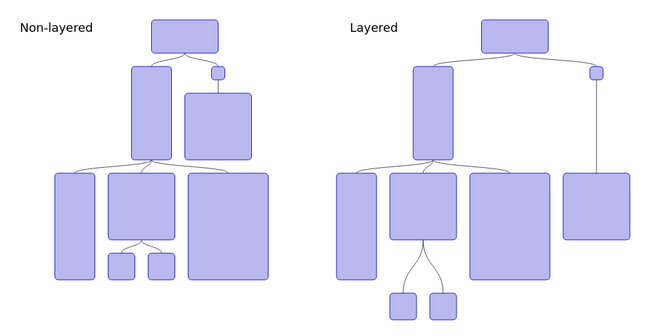](https://elm-visualization.netlify.app/LayeredTree/)\n\nPassing this option causes each \"layer\" (i.e. nodes in the tree that have the same number of ancestor nodes)\nto be layed out with the same y value. This makes the layers much more emphasized (if you are for instance\nvisualizing the organization of an army unit, then this might neatly show the rank of each member) at the cost\nof needing more space.\n\nThis only makes a difference if `nodeSize` returns different heights for different children.\n\n","type":"Hierarchy.Attribute a { b | layered : Hierarchy.Supported }"},{"name":"nodeSize","comment":" Sets the size of the actual node to be layed out. This will be the actual\nsize if the `size` option isn't passed, otherwise this size will get proportionally\nscaled (preserving aspect ratio).\n\nThe default size of a node is `( 1, 1 )`.\n\n","type":"(a -> ( Basics.Float, Basics.Float )) -> Hierarchy.Attribute a { b | nodeSize : Hierarchy.Supported }"},{"name":"none","comment":" Attribute that doesn't affect the settings at all. Can be useful when settings are produced conditionally:\n\n [ Hierarchy.size 230 520\n , if doLayered then\n Hierarchy.layered\n\n else\n Hierarchy.none\n ]\n\n","type":"Hierarchy.Attribute a b"},{"name":"padding","comment":" Sets the distances between nodes. For treemaps, this is a shortcut to setting both paddingInner and paddingOuter.\n","type":"(a -> Basics.Float) -> Hierarchy.Attribute a { b | padding : Hierarchy.Supported }"},{"name":"paddingBottom","comment":" The bottom padding is used to separate the bottom edge of a node from its children.\n","type":"(a -> Basics.Float) -> Hierarchy.Attribute a { b | paddingOuter : Hierarchy.Supported }"},{"name":"paddingInner","comment":" The inner padding is used to separate a node’s adjacent children.\n","type":"(a -> Basics.Float) -> Hierarchy.Attribute a { b | paddingInner : Hierarchy.Supported }"},{"name":"paddingLeft","comment":" The left padding is used to separate the left edge of a node from its children.\n","type":"(a -> Basics.Float) -> Hierarchy.Attribute a { b | paddingOuter : Hierarchy.Supported }"},{"name":"paddingOuter","comment":" Sets `paddingLeft`, `paddingRight`, `paddingTop` and `paddingBottom` in one go.\n","type":"(a -> Basics.Float) -> Hierarchy.Attribute a { b | paddingOuter : Hierarchy.Supported }"},{"name":"paddingRight","comment":" The right padding is used to separate the right edge of a node from its children.\n","type":"(a -> Basics.Float) -> Hierarchy.Attribute a { b | paddingOuter : Hierarchy.Supported }"},{"name":"paddingTop","comment":" The top padding is used to separate the top edge of a node from its children.\n","type":"(a -> Basics.Float) -> Hierarchy.Attribute a { b | paddingOuter : Hierarchy.Supported }"},{"name":"parentChildMargin","comment":" The vertical distance between a parent and a child in a tree.\n","type":"Basics.Float -> Hierarchy.Attribute a { b | parentChildMargin : Hierarchy.Supported }"},{"name":"partition","comment":" The partition layout produces adjacency diagrams: a space-filling variant of a node-link tree diagram. Rather than drawing a link between parent and child in the hierarchy, nodes are drawn as solid areas (either arcs or rectangles), and their placement relative to other nodes reveals their position in the hierarchy. The size of the nodes encodes a quantitative dimension that would be difficult to show in a node-link diagram.\n\n[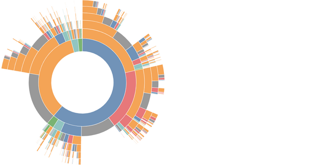](https://elm-visualization.netlify.app/Sunburst/)\n\n","type":"List.List (Hierarchy.Attribute a { padding : Hierarchy.Supported, size : Hierarchy.Supported }) -> (a -> Basics.Float) -> Tree.Tree a -> Tree.Tree { x : Basics.Float, y : Basics.Float, width : Basics.Float, height : Basics.Float, value : Basics.Float, node : a }"},{"name":"peerMargin","comment":" The horizontal distance between nodes layed out next to each other.\n","type":"Basics.Float -> Hierarchy.Attribute a { b | peerMargin : Hierarchy.Supported }"},{"name":"size","comment":" Sets the size of the entire layout. For most layouts omitting this option will cause it to have a default size of 1.\n","type":"Basics.Float -> Basics.Float -> Hierarchy.Attribute a { b | size : Hierarchy.Supported }"},{"name":"slice","comment":" Divides the rectangular area **vertically**. The children are positioned in order, starting with the top edge (y0) of the given rectangle.\n\nIf the sum of the children’s values is less than the specified node’s value (i.e., if the specified node has a non-zero internal value), the remaining empty space will be positioned on the bottom edge (y1) of the given rectangle.\n\n","type":"Hierarchy.TilingMethod"},{"name":"sliceDice","comment":" If the depth is odd, delegates to `slice`; otherwise delegates to `dice`.\n","type":"Hierarchy.TilingMethod"},{"name":"squarify","comment":" Implements the squarified treemap algorithm by [Bruls et al.](https://www.win.tue.nl/~vanwijk/stm.pdf), which seeks to produce rectangles of a given aspect ratio, in this case the golden ratio φ = (1 + sqrt(5)) / 2.\n","type":"Hierarchy.TilingMethod"},{"name":"squarifyRatio","comment":" Implements the squarified treemap algorithm by [Bruls et al.](https://www.win.tue.nl/~vanwijk/stm.pdf), which seeks to produce rectangles of the given aspect ratio. The ratio must be specified as a number greater than or equal to one. Note that the orientation of the generated rectangles (tall or wide) is not implied by the ratio; for example, a ratio of two will attempt to produce a mixture of rectangles whose width:height ratio is either 2:1 or 1:2. (However, you can approximately achieve this result by generating a square treemap at different dimensions, and then stretching the treemap to the desired aspect ratio.) Furthermore, the specified ratio is merely a hint to the tiling algorithm; the rectangles are not guaranteed to have the specified aspect ratio.\n","type":"Basics.Float -> Hierarchy.TilingMethod"},{"name":"tidy","comment":" Produces a tidy node-link diagram of a tree, based on a linear time algorithm by [van der Ploeg](https://citeseerx.ist.psu.edu/document?repid=rep1&type=pdf&doi=d45f66231e053590c64c9d901fb7b028dbc5c923).\n\n[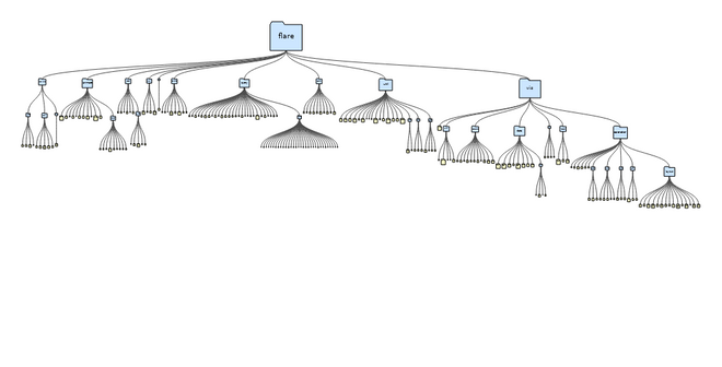](https://elm-visualization.netlify.app/TidyTree/)\n\n","type":"List.List (Hierarchy.Attribute a { size : Hierarchy.Supported, nodeSize : Hierarchy.Supported, layered : Hierarchy.Supported, parentChildMargin : Hierarchy.Supported, peerMargin : Hierarchy.Supported }) -> Tree.Tree a -> Tree.Tree { height : Basics.Float, node : a, width : Basics.Float, x : Basics.Float, y : Basics.Float }"},{"name":"tile","comment":" Sets the tiling method to be used. The default is `squarify`.\n","type":"Hierarchy.TilingMethod -> Hierarchy.Attribute a { b | tile : Hierarchy.Supported }"},{"name":"treemap","comment":" A treemap recursively subdivides area into rectangles according to each node’s associated value. This implementation supports an extensible tiling method.\n\n[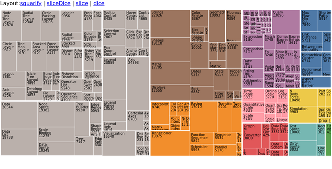](https://elm-visualization.netlify.app/Treemap/)\n\n","type":"List.List (Hierarchy.Attribute a { padding : Hierarchy.Supported, paddingInner : Hierarchy.Supported, paddingOuter : Hierarchy.Supported, tile : Hierarchy.Supported, size : Hierarchy.Supported }) -> (a -> Basics.Float) -> Tree.Tree a -> Tree.Tree { x : Basics.Float, y : Basics.Float, width : Basics.Float, height : Basics.Float, value : Basics.Float, node : a }"}],"binops":[]},{"name":"Histogram","comment":" A histogram is an accurate graphical representation of the distribution of\nnumerical data. It is an estimate of the probability distribution of a continuous\nvariable (quantitative variable)\n\n[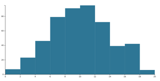](https://elm-visualization.netlify.app/HistogramChart/)\n\nTo compute a histogram, one first configures a Histogram Generator and then uses\nit to compute a histogram. Histograms can then be visualized in a variety of ways,\nfor example using Svg rects and linear scales.\n\n\n### Configuring a Generator\n\n@docs HistogramGenerator, float, generator, custom, withDomain\n\n\n### Computing a Histogram\n\n@docs Bin, compute\n\n\n### Thresholds\n\n@docs Threshold, sturges, steps, binCount\n\n","unions":[{"name":"HistogramGenerator","comment":" Represents configuration to compute a histogram from a list of arbitrary data.\n\nHowever, to compute a histogram, the data must be made comparable, this is typically done\nthrough a conversion to a `Float`, however any `comparable` type will do.\n\n","args":["a","comparable"],"cases":[]}],"aliases":[{"name":"Bin","comment":" A bin holding data. All of the data falling into the bin is available in `values`. Each of the\n`values` (when transformed to a comparable) falls between `x0` and `x1`. The number of elements in the\nbin is available as `length`, which is equivalent to (but faster then) `List.length values`.\n","args":["a","comparable"],"type":"{ x0 : comparable, x1 : comparable, values : List.List a, length : Basics.Int }"},{"name":"Threshold","comment":" A function that computes threshold values separating the individual bins. It is passed a function that\ncan convert values to comparables, the list of all valus and the extent (i.e. smallest and largest value).\nNote that the smallest and largest value may be the same, however the list of all values is guaranteed not to\nbe empty.\n\nIt must return a list of boundary values that separate the bins. If you wish to have `n` bins, this should\nreturn `n-1` thresholds.\n\n","args":["a","comparable"],"type":"(a -> comparable) -> List.List a -> ( a, a ) -> List.List comparable"}],"values":[{"name":"binCount","comment":" Computes appropriate threshold values given an extent and the desired number of bins. Useful for implementing\nyour custom `Threshold` values when you have a way to compute the desired number of bins.\n","type":"( Basics.Float, Basics.Float ) -> Basics.Int -> List.List Basics.Float"},{"name":"compute","comment":" Given some data and a configured HistogramGenerator, computes the binning of the data.\n\nIf the data is empty, returns an empty list.\n\n","type":"List.List a -> Histogram.HistogramGenerator a comparable -> List.List (Histogram.Bin a comparable)"},{"name":"custom","comment":" Create a custom generator by supplying your own threshold function and a mapping function.\n","type":"Histogram.Threshold a comparable -> (a -> comparable) -> Histogram.HistogramGenerator a comparable"},{"name":"float","comment":" Create a histogram generator that takes float data and uses Sturges' formula for thresholding.\n","type":"Histogram.HistogramGenerator Basics.Float Basics.Float"},{"name":"generator","comment":" Make histograms with arbitrary data passing in a function that converts the data to a Float.\n\nThis is pretty similar to using `Histogram.float` and `List.map`ing your data in advance, however\nhere you will have access to the original data in the bins if needed for further analysis.\n\n","type":"(a -> Basics.Float) -> Histogram.HistogramGenerator a Basics.Float"},{"name":"steps","comment":" For creating an appropriate Threshold value if you already have appropriate\nThreshold values (i.e. from `Scale.ticks`).\n","type":"List.List a -> Histogram.Threshold a comparable"},{"name":"sturges","comment":" Returns the threshold values according to [Sturges’ formula](https://en.wikipedia.org/wiki/Histogram#Mathematical_definition).\nThis is a decent default value, however it implicitly assumes an approximately normal distribution and may perform poorly\nif you have less than 30 data points.\n","type":"(a -> Basics.Float) -> List.List a -> ( a, a ) -> List.List Basics.Float"},{"name":"withDomain","comment":" Set the domain for the HistogramGenerator. All values falling outside the domain will be ignored.\n","type":"( a, a ) -> Histogram.HistogramGenerator a comparable -> Histogram.HistogramGenerator a comparable"}],"binops":[]},{"name":"Interpolation","comment":" This module provides a variety of interpolation methods for blending between two values.\nWhile primitives for numbers, colors and lists are provided, the library focuses on composition\nso that you can build interpolators for your own custom datatypes.\n\n@docs Interpolator\n\n\n### Primitive interpolators\n\n@docs float, int, step, rgb, rgbWithGamma, hsl, hslLong, lab, hcl, hclLong\n\n\n### Composition\n\n@docs map, map2, map3, map4, map5, piecewise, tuple\n\n\n### Lists\n\n@docs inParallel, staggeredWithParallelism, list, ListCombiner, combineParallel\n\n\n### Advanced\n\n@docs pointAlongPath\n\n\n## Helpers\n\n@docs samples\n\n","unions":[{"name":"ListCombiner","comment":" ","args":[],"cases":[["CombineParallel",[]]]}],"aliases":[{"name":"Interpolator","comment":" An interpolator is merely a function that takes a float parameter `t` roughly in the range [0..1].\n0 would represent the \"before\" value, 1 the after value and values in between are the values in between.\n\nNote: Sometimes the range of the interpolator can go slightly above or below zero - this is useful for some\nanimation techniques. If this is not suitable for your data type, remember to clamp the values as necessary.\n\n","args":["a"],"type":"Basics.Float -> a"}],"values":[{"name":"combineParallel","comment":" Runs all the list interpolations in parallel.\n","type":"Interpolation.ListCombiner"},{"name":"float","comment":" Interpolates between the two provided float values.\n\n myInterpolator : Interpolator Float\n myInterpolator = Interpolation.float 5 17\n\n myInterpolator 0.2 -- 7.4\n myInterpolator 0.5 -- 11\n\n","type":"Basics.Float -> Basics.Float -> Interpolation.Interpolator Basics.Float"},{"name":"hcl","comment":" Interpolates between two Color values using the [CIE Lch(ab)](https://en.wikipedia.org/wiki/HCL_color_space) color space.\n","type":"Color.Color -> Color.Color -> Interpolation.Interpolator Color.Color"},{"name":"hclLong","comment":" Like hcl, but does not use the shortest path between hues.\n","type":"Color.Color -> Color.Color -> Interpolation.Interpolator Color.Color"},{"name":"hsl","comment":" Interpolates between two Color values using the HSL color space. It will always take the shortest path between the target hues.\n","type":"Color.Color -> Color.Color -> Interpolation.Interpolator Color.Color"},{"name":"hslLong","comment":" Like `Interpolation.hsl`, but does not use the shortest path between hues.\n","type":"Color.Color -> Color.Color -> Interpolation.Interpolator Color.Color"},{"name":"inParallel","comment":" This will run all of the interpolators provided in parallel.\n\nCan be handy for constructing complex interpolations in conjuction with `List.map2`:\n\n before : List Float\n before =\n [ 3, 4, 7, 8 ]\n\n after : List Float\n after =\n [ 6, 4, 1, 9 ]\n\n myInterpolator0 : Interpolator (List Float)\n myInterpolator0 =\n List.map2 Interpolation.float before after\n |> Interpolation.inParallel\n\n myInterpolator0 0 --> [ 3, 4, 7, 8 ]\n myInterpolator0 0.5 --> [ 4.5, 4, 4, 8.5]\n myInterpolator0 1 --> [ 6, 4, 1, 9 ]\n\n","type":"List.List (Interpolation.Interpolator a) -> Interpolation.Interpolator (List.List a)"},{"name":"int","comment":" Interpolates between ints.\n","type":"Basics.Int -> Basics.Int -> Interpolation.Interpolator Basics.Int"},{"name":"lab","comment":" Interpolates between two Color values using the [CIELAB](https://en.wikipedia.org/wiki/CIELAB_color_space) color space, that is more perceptually linear than other color spaces.\nPerceptually linear means that a change of the same amount in a color value should produce a change of about the same visual importance.\nThis property makes it ideal for accurate visual encoding of data.\n","type":"Color.Color -> Color.Color -> Interpolation.Interpolator Color.Color"},{"name":"list","comment":" This is an interpolator for lists. It is quite complex and should be used if these conditions hold:\n\n1. You need to interpolate additions, removals and changes.\n2. Each item in the list has some notion of identity, for example an `.id` member, which is `comparable`.\n3. You have a way to deal with positions in the list being somewhat muddy during the transition (e.g. if an item is being created at the same position a different item is being removed, while adjacent items are switching position, then the exact order of items will be arbitrary during the interpolation).\n\nThe first argument is a configuration record. It has the following keys:\n\n - `id : a -> comparable` is a function that retrieves some sort of identifier for each item in the list. It is used to figure out if an item is added, removed, or modified.\n - `add : a -> Interpolator a` will be invoked for each item being added to the list.\n - `remove : a -> Interpolator a` will be invoked for each item disappearing from the list. Note that the item won't actually be removed from the list until `t = 1`, so you will most likely want to make the item disappear visually.\n - `change : a -> a -> Interpolator a` is called for an item where the `id` matches for both lists, but which are not equal.\n - `combine : ListCombiner` configures a strategy that orchestrates all the interpolations created. At the moment only 'combineParallel' is supported, but staggered transitions will be supported in the future.\n\n","type":"{ add : a -> Interpolation.Interpolator a, remove : a -> Interpolation.Interpolator a, change : a -> a -> Interpolation.Interpolator a, id : a -> comparable, combine : Interpolation.ListCombiner } -> List.List a -> List.List a -> Interpolation.Interpolator (List.List a)"},{"name":"map","comment":" Transform values from another interpolator.\n\nNote: This function is provided as a convenience, since thinking in `mapN` is pretty natural for Elm developers (and\nworks well in pipelines). However, keep in mind that this function is literally an alias for `<<`.\n\n","type":"(a -> b) -> Interpolation.Interpolator a -> Interpolation.Interpolator b"},{"name":"map2","comment":" Combine two interpolators, combining them with the given function.\n\n type alias Coords =\n ( Float, Float )\n\n interpolateCoords : Coords -> Coords -> Interpolator Coords\n interpolateCoords ( x1, y1 ) ( x2, y2 ) =\n Interpolation.map2\n Tuple.pair\n (Interpolation.float x1 x2)\n (Interpolation.float y1 y2)\n\n","type":"(a -> b -> c) -> Interpolation.Interpolator a -> Interpolation.Interpolator b -> Interpolation.Interpolator c"},{"name":"map3","comment":" ","type":"(a -> b -> c -> d) -> Interpolation.Interpolator a -> Interpolation.Interpolator b -> Interpolation.Interpolator c -> Interpolation.Interpolator d"},{"name":"map4","comment":" ","type":"(a -> b -> c -> d -> e) -> Interpolation.Interpolator a -> Interpolation.Interpolator b -> Interpolation.Interpolator c -> Interpolation.Interpolator d -> Interpolation.Interpolator e"},{"name":"map5","comment":" ","type":"(a -> b -> c -> d -> e -> f) -> Interpolation.Interpolator a -> Interpolation.Interpolator b -> Interpolation.Interpolator c -> Interpolation.Interpolator d -> Interpolation.Interpolator e -> Interpolation.Interpolator f"},{"name":"piecewise","comment":" Returns a piecewise interpolator, composing interpolators for each adjacent pair of values.\n\nFor example:\n\n myInterpolator : Interpolator Int\n myInterpolator =\n Interpolation.piecewise Interpolation.int 6 [ 10, -2 ]\n\n myInterpolator 0 --> 6\n myInterpolator 0.25 --> 8\n myInterpolator 0.5 --> 10\n myInterpolator 0.75 --> 4\n myInterpolator 1 --> -2\n\n","type":"(a -> a -> Interpolation.Interpolator a) -> a -> List.List a -> Interpolation.Interpolator a"},{"name":"pointAlongPath","comment":" A somewhat elaborate interpolator that gives points along an arbitrary path, where at `t=0` this will give the first point in the path,\nand at `t=1` gives the last. If overshot, will give points along the tangent at these points.\n\nWill give the origin point if the path is empty or invalid (generally you should check somewhere earlier if there is a possibility of that).\n\nPerformance note: this function does a fair amount of work when the interpolator is being constructed, so that later when it is called with\nthe `t` parameter it can be rather efficient. Therefore it is more efficient to partially apply this with a path in a static context or store\nthe partially applied function in a model.\n\n","type":"Path.Path -> Interpolation.Interpolator ( Basics.Float, Basics.Float )"},{"name":"rgb","comment":" Interpolates between two Color values using the sRGB color space.\n","type":"Color.Color -> Color.Color -> Interpolation.Interpolator Color.Color"},{"name":"rgbWithGamma","comment":" Interpolates between two Color values using the sRGB color space using [gamma correction](https://web.archive.org/web/20160112115812/http://www.4p8.com/eric.brasseur/gamma.html).\n","type":"Basics.Float -> Color.Color -> Color.Color -> Interpolation.Interpolator Color.Color"},{"name":"samples","comment":" Returns a list of uniformly spaced samples from the specified interpolator. The first sample is always at t = 0, and the last sample is always at t = 1. This can be useful in generating a fixed number of samples from a given interpolator.\n\nCan be quite handy when debugging interpolators or as a way to create a quantize scale.\n\n","type":"Basics.Int -> Interpolation.Interpolator a -> List.List a"},{"name":"staggeredWithParallelism","comment":" Combines a bunch of interpolators with a controlled amount of parallelism.\n\nLet's illustrate what we mean by showing an example:\n\n interpolate : Float -> Interpolator (List Int)\n interpolate parallelism =\n List.repeat 5 (Interpolation.int 0 8)\n |> Interpolation.staggeredWithParallelism parallelism\n\nNow when the parallelism is 1, we will run each interpolator when the previous one concludes:\n\n Interpolation.samples 11 (interpolate 1)\n --> [ [ 0, 0, 0, 0, 0 ]\n --> , [ 4, 0, 0, 0, 0 ]\n --> , [ 8, 0, 0, 0, 0 ]\n --> , [ 8, 4, 0, 0, 0 ]\n --> , [ 8, 8, 0, 0, 0 ]\n --> , [ 8, 8, 4, 0, 0 ]\n --> , [ 8, 8, 8, 0, 0 ]\n --> , [ 8, 8, 8, 4, 0 ]\n --> , [ 8, 8, 8, 8, 0 ]\n --> , [ 8, 8, 8, 8, 4 ]\n --> , [ 8, 8, 8, 8, 8 ]\n --> ]\n\nIf we set it to 2, we will start each interpolator approximately halfway through the previous one:\n\n Interpolation.samples 11 (interpolate 2)\n --> [ [ 0, 0, 0, 0, 0 ]\n --> , [ 2, 0, 0, 0, 0 ]\n --> , [ 5, 1, 0, 0, 0 ]\n --> , [ 7, 3, 0, 0, 0 ]\n --> , [ 8, 6, 2, 0, 0 ]\n --> , [ 8, 8, 4, 0, 0 ]\n --> , [ 8, 8, 6, 2, 0 ]\n --> , [ 8, 8, 8, 5, 1 ]\n --> , [ 8, 8, 8, 7, 3 ]\n --> , [ 8, 8, 8, 8, 6 ]\n --> , [ 8, 8, 8, 8, 8 ]\n --> ]\n\nIf we set it to 1/2, we will wait approximately the time a single interpolator runs after each run doing nothing (slightly more samples so it's easier to see what's going on):\n\n Interpolation.samples 16 (interpolate 0.5)\n --> [ [ 0, 0, 0, 0, 0 ]\n --> , [ 5, 0, 0, 0, 0 ]\n --> , [ 8, 0, 0, 0, 0 ]\n --> , [ 8, 0, 0, 0, 0 ]\n --> , [ 8, 3, 0, 0, 0 ]\n --> , [ 8, 8, 0, 0, 0 ]\n --> , [ 8, 8, 0, 0, 0 ]\n --> , [ 8, 8, 2, 0, 0 ]\n --> , [ 8, 8, 6, 0, 0 ]\n --> , [ 8, 8, 8, 0, 0 ]\n --> , [ 8, 8, 8, 0, 0 ]\n --> , [ 8, 8, 8, 5, 0 ]\n --> , [ 8, 8, 8, 8, 0 ]\n --> , [ 8, 8, 8, 8, 0 ]\n --> , [ 8, 8, 8, 8, 3 ]\n --> , [ 8, 8, 8, 8, 8 ]\n --> ]\n\nAs parallelism approaches infinity, than this will behave like `Interpolation.inParallel`.\n\nIf thinking about this in terms of parallelism doesn't feel natural, you may appreciate `Transition.stagger` which deals\nwith durations and delays instead.\n\n","type":"Basics.Float -> List.List (Interpolation.Interpolator a) -> Interpolation.Interpolator (List.List a)"},{"name":"step","comment":" Interpolate between arbitrary values by just showing them in sequence.\n\nThe list is provided is passed as head and tail seperately, to avoid needing to handle the empty list case.\n\n type StageOfGrief\n = Denial\n | Anger\n | Bargaining\n | Depression\n | Acceptance\n\n griefInterpolator : Interpolator StageOfGrief\n griefInterpolator =\n Interpolation.step Denial\n [ Anger\n , Bargaining\n , Depression\n , Acceptance\n ]\n\n griefInterpolator 0 --> Denial\n griefInterpolator 0.5 --> Bargaining\n griefInterpolator 1.1 --> Acceptance\n\n","type":"a -> List.List a -> Interpolation.Interpolator a"},{"name":"tuple","comment":" Composes interpolators around a tuple. This is a convenience function for the common case of 2 element tuples.\n\nYou can for example define an interpolator for a position:\n\n interpolatePosition : ( Float, Float ) -> ( Float, Float ) -> Interpolator ( Float, Float )\n interpolatePosition =\n Interpolation.tuple Interpolation.float Interpolation.float\n\n","type":"(a -> a -> Interpolation.Interpolator a) -> (b -> b -> Interpolation.Interpolator b) -> ( a, b ) -> ( a, b ) -> Interpolation.Interpolator ( a, b )"}],"binops":[]},{"name":"Scale","comment":" Scales are a convenient abstraction for a fundamental task in visualization:\nmapping a dimension of abstract data to a visual representation. Although most\noften used for position-encoding quantitative data, such as mapping a measurement\nin meters to a position in pixels for dots in a scatterplot, scales can represent\nvirtually any visual encoding, such as diverging colors, stroke widths, or symbol\nsize. Scales can also be used with virtually any type of data, such as named\ncategorical data or discrete data that requires sensible breaks.\n\nFor [continuous](#ContinuousScale) quantitative data, you typically want a [linear scale](#linear). (For time\nseries data, a [time scale](#time).) If the distribution calls for it, consider\ntransforming data using a [log scale](#log). A [quantize scale](#QuantizeScale) may aid\ndifferentiation by rounding continuous data to a fixed set of discrete values.\n\nFor discrete ordinal (ordered) or categorical (unordered) data, an [ordinal scale](#OrdinalScale)\nspecifies an explicit mapping from a set of data values to a corresponding set\nof visual attributes (such as colors). The related [band](#BandScale) scale is\nuseful for position-encoding ordinal data, such as bars in a bar chart.\n\nScales have no intrinsic visual representation. However, most scales can generate\nand format ticks for reference marks to aid in the construction of [axes](Axis).\n\n\n### Scales\n\n - [Continuous](#ContinuousScale) ([linear](#linear), [power](#power), [log](#log), [symlog](#symlog), [identity](#identity), [time](#time), [radial](#radial))\n - [Sequential](#SequentialScale)\n - [Diverging](#DivergingScale)\n - [Quantize](#QuantizeScale)\n - [Quantile](#QuantileScale)\n - [Threshold](#ThresholdScale)\n - [Ordinal](#OrdinalScale) ([Band](#BandScale), [Point](#point))\n\n@docs Scale\n\n\n# Continuous Scales\n\n@docs ContinuousScale, linear, power, log, symlog, identity, time, radial\n\n\n# Sequential Scales\n\nSequential scales are similar to continuous scales in that they map a continuous,\nnumeric input domain to a continuous output range. However, unlike continuous\nscales, the output range of a sequential scale is fixed by its interpolator function.\n\n@docs SequentialScale, sequential, sequentialLog, sequentialSymlog, sequentialPower\n\nYou can find some premade color interpolators in the [Scale.Color](Scale-Color) module.\n\n\n# Diverging Scales\n\nDiverging scales, like sequential scales, are similar to continuous scales in that they\nmap a continuous, numeric input domain to a continuous output range. However, unlike\ncontinuous scales, the input domain and output range of a diverging scale always has exactly\nthree elements, and the output range is specified as an interpolator rather than an array of\nvalues. These scales do not expose invert and interpolate methods.\n\n@docs DivergingScale, diverging, divergingLog, divergingSymlog, divergingPower\n\n\n# Quantize Scales\n\nQuantize scales are similar to linear scales, except they use a discrete rather\nthan continuous range. The continuous input domain is divided into uniform\nsegments based on the number of values in (i.e., the cardinality of) the output\nrange. Each range value y can be expressed as a quantized linear function of the\ndomain value `x`: `y = m round(x) + b`.\n\n@docs QuantizeScale, quantize\n\n\n# Quantile Scales\n\nQuantile scales map a sampled input domain to a discrete range. The number of values\nin the output range determines the number of quantiles that will be computed from the domain.\nTo compute the quantiles, the domain is sorted, and treated as a population of discrete values;\nsee [`Statistics.quantile`](https://package.elm-lang.org/packages/gampleman/elm-visualization/latest/Statistics#quantile).\n\n@docs QuantileScale, quantile\n\n\n# Threshold Scales\n\nThreshold scales are similar to quantize scales, except they allow you to map arbitrary\nsubsets of the domain to discrete values in the range. The input domain is still continuous,\nand divided into slices based on a set of threshold values.\n\n@docs ThresholdScale, threshold\n\n\n# Ordinal Scales\n\nUnlike continuous scales, ordinal scales have a discrete domain and range. For\nexample, an ordinal scale might map a set of named categories to a set of colors,\nor determine the horizontal positions of columns in a column chart.\n\n@docs OrdinalScale, ordinal\n\nYou can find some premade color schemes in the [Scale.Color](Scale-Color) module.\n\n\n## Band Scales\n\nBand scales are like ordinal scales except the output range is continuous and\nnumeric. Discrete output values are automatically computed by the scale by\ndividing the continuous range into uniform bands. Band scales are typically used\nfor bar charts with an ordinal or categorical dimension.\n\n@docs BandScale, band, BandConfig, defaultBandConfig\n\n\n## Point Scales\n\nPoint scales are a variant of band scales with the bandwidth fixed to zero.\nPoint scales are typically used for scatterplots with an ordinal or categorical dimension.\n\n@docs point, PointConfig, defaultPointConfig\n\n\n# Operations\n\nThese functions take Scales and do something with them. Check the docs of each scale type to see which operations it supports.\n\n@docs convert, invert, invertExtent, domain, range, rangeExtent, ticks, tickFormat, clamp, nice, quantiles, bandwidth, toRenderable\n\n","unions":[{"name":"Scale","comment":" This API is highly polymorphic as each scale has different functions supported.\nThis is still done in a convenient and type-safe manner, however the cost is\na certain ugliness and complexity of the type signatures. For this reason after the type alias of each scale, the supported functions are listed along with a more specialized type signature appropriate for that scale type.\n\n**Note:** As a convention, the scales typically take arguments in a `range -> domain` order. This may seem somewhat counterinutive, as scales map a domain onto a range, but it is quite common to need to compute the domain, but know the range statically, so this argument order works much better for composition.\n\nIf you're new to this, I recommend ignoring the types of the type aliases and of the operations and just look at these listings.\n\n","args":["scaleSpec"],"cases":[]}],"aliases":[{"name":"BandConfig","comment":" Configuration options for deciding how bands are partioned,\n\n\n### `.paddingInner : Float`\n\nThe inner padding determines the ratio (so the value must be in\nthe range [0, 1]) of the range that is reserved for blank space\nbetween bands.\n\n\n### `.paddingOuter : Float`\n\nThe outer padding determines the ratio (so the value must be in\nthe range [0, 1]) of the range that is reserved for blank space\nbefore the first band and after the last band.\n\n\n### `.align : Float`\n\nThe alignment determines how any leftover unused space in the range\nis distributed. A value of 0.5 indicates that the leftover space\nshould be equally distributed before the first band and after the last\nband; i.e., the bands should be centered within the range. A value\nof 0 or 1 may be used to shift the bands to one side, say to position\nthem adjacent to an axis.\n\n","args":[],"type":"{ paddingInner : Basics.Float, paddingOuter : Basics.Float, align : Basics.Float }"},{"name":"BandScale","comment":" Type alias for a band scale. These transform an arbitrary `List a`\nto a continous (Float, Float) by uniformely partitioning the range.\n\nBand scales support the following operations:\n\n - [`convert : BandScale a -> a -> Float`](#convert)\n - [`domain : BandScale a -> List a`](#domain)\n - [`range : Bandscale a -> (Float, Float)`](#range)\n - [`bandwidth : Bandscale a -> Float`](#bandwidth)\n - [`toRenderable : (a -> String) -> BandScale a -> RenderableScale a`](#toRenderable)\n\n","args":["a"],"type":"Scale.Scale { domain : List.List a, range : ( Basics.Float, Basics.Float ), convert : List.List a -> ( Basics.Float, Basics.Float ) -> a -> Basics.Float, bandwidth : Basics.Float }"},{"name":"ContinuousScale","comment":" Maps a `(inp, inp)` **domain** to a\n`(Float, Float)` **range** (this will be either `(Float, Float)` or `(Time.Posix, Time.Posix)`.)\n\nContinuous scales support the following operations:\n\n - [`convert : ContinuousScale inp -> inp -> Float`](#convert)\n - [`invert : ContinuousScale inp -> Float -> inp`](#invert)\n - [`domain : ContinuousScale inp -> (inp, inp)`](#domain)\n - [`range : ContinuousScale inp -> (Float, Float)`](#range)\n - [`rangeExtent : ContinuousScale inp -> (Float, Float)`](#rangeExtent) (which is in this case just an alias for `range`)\n - [`ticks : ContinuousScale inp -> Int -> List inp`](#ticks)\n - [`tickFormat : ContinuousScale inp -> Int -> inp -> String`](#tickFormat)\n - [`clamp : ContinuousScale inp -> ContinuousScale inp`](#clamp)\n - [`nice : Int -> ContinuousScale inp -> ContinuousScale inp`](#nice)\n\n","args":["inp"],"type":"Scale.Scale { domain : ( inp, inp ), range : ( Basics.Float, Basics.Float ), convert : ( inp, inp ) -> ( Basics.Float, Basics.Float ) -> inp -> Basics.Float, invert : ( inp, inp ) -> ( Basics.Float, Basics.Float ) -> Basics.Float -> inp, ticks : ( inp, inp ) -> Basics.Int -> List.List inp, tickFormat : ( inp, inp ) -> Basics.Int -> inp -> String.String, nice : ( inp, inp ) -> Basics.Int -> ( inp, inp ), rangeExtent : ( inp, inp ) -> ( Basics.Float, Basics.Float ) -> ( Basics.Float, Basics.Float ) }"},{"name":"DivergingScale","comment":" This transforms a continuous `(Float, Float, Float)`\ndomain to an arbitrary range `a` defined by the interpolator function `Float -> a`, where the `Float` goes from 0 to 1.\n\nThe middle float is the neutral or zero point.\n\nDiverging scales support the following operations:\n\n - [`convert : DivergingScale a -> Float -> a`](#convert)\n - [`domain : DivergingScale a -> (Float, Float)`](#domain)\n - [`range : DivergingScale a -> Float -> a`](#range)\n\n","args":["a"],"type":"Scale.Scale { domain : ( Basics.Float, Basics.Float, Basics.Float ), range : Basics.Float -> a, convert : ( Basics.Float, Basics.Float, Basics.Float ) -> (Basics.Float -> a) -> Basics.Float -> a }"},{"name":"OrdinalScale","comment":" Type alias for ordinal scales. These transform an arbitrary\n`List a` domain to an arbitrary list `List b`, where the mapping\nis based on order.\n\nOrdinal scales support the following operations:\n\n - [`convert : OrdinalScale a b -> a -> Maybe b`](#convert)\n\n Note that this returns a `Maybe` value in the case when you pass a value that isn't in the domain.\n\n - [`domain : OrdinalScale a b -> List a`](#domain)\n\n - [`range : OrdinalScale a b -> List b`](#range)\n\n","args":["a","b"],"type":"Scale.Scale { domain : List.List a, range : List.List b, convert : List.List a -> List.List b -> a -> Maybe.Maybe b }"},{"name":"PointConfig","comment":" Configuration options for Point scales. See [BandConfig](#BandConfig) for details, as `align` works exactly the same, and `padding` is equivalent to `paddingOuter`.\n","args":[],"type":"{ padding : Basics.Float, align : Basics.Float }"},{"name":"QuantileScale","comment":" These transform a `List Float` domain\nto an arbitrary non-empty list `(a, List a)`. However, internally this gets converted to a sorted Array.\n\nQuantile scales support the following operations:\n\n - [`convert : QuantileScale a -> Float -> a`](#convert)\n - [`invertExtent : QuantileScale a -> a -> Maybe (Float, Float)`](#invertExtent)\n - [`domain : QuantileScale a -> List Float`](#domain)\n - [`range : QuantileScale a -> Array a`](#range)\n - [`quantiles : QuantileScale a -> List Float`](#quantiles)\n\n","args":["a"],"type":"Scale.Scale { domain : List.List Basics.Float, range : Array.Array a, convert : List.List Basics.Float -> Array.Array a -> Basics.Float -> a, invertExtent : List.List Basics.Float -> Array.Array a -> a -> Maybe.Maybe ( Basics.Float, Basics.Float ), quantiles : List.List Basics.Float }"},{"name":"QuantizeScale","comment":" These transform a `(Float, Float)` domain\nto an arbitrary non-empty list `(a, List a)`.\n\nQuantize scales support the following operations:\n\n - [`convert : QuantizeScale a -> Float -> a`](#convert),\n - [`invertExtent : QuantizeScale a -> a -> Maybe (Float, Float)`](#invertExtent)\n - [`domain : QuantizeScale a -> (Float, Float)`](#domain)\n - [`range : QuantizeScale a -> (a, List a)`](#range),\n - [`rangeExtent : QuantizeScale a -> (a, a)`](#rangeExtent)\n - [`ticks : QuantizeScale a -> Int -> List Float`](#ticks)\n - [`tickFormat : QuantizeScale a -> Int -> Float -> String`](#tickFormat)\n - [`nice : Int -> QuantizeScale a -> QuantizeScale a`](#nice)\n - [`clamp : QuantizeScale a -> QuantizeScale a`](#clamp)\n\n","args":["a"],"type":"Scale.Scale { domain : ( Basics.Float, Basics.Float ), range : ( a, List.List a ), convert : ( Basics.Float, Basics.Float ) -> ( a, List.List a ) -> Basics.Float -> a, invertExtent : ( Basics.Float, Basics.Float ) -> ( a, List.List a ) -> a -> Maybe.Maybe ( Basics.Float, Basics.Float ), ticks : ( Basics.Float, Basics.Float ) -> ( a, List.List a ) -> Basics.Int -> List.List Basics.Float, tickFormat : ( Basics.Float, Basics.Float ) -> Basics.Int -> Basics.Float -> String.String, nice : ( Basics.Float, Basics.Float ) -> Basics.Int -> ( Basics.Float, Basics.Float ), rangeExtent : ( Basics.Float, Basics.Float ) -> ( a, List.List a ) -> ( a, a ) }"},{"name":"SequentialScale","comment":" This transforms a continuous `(Float, Float)`\ndomain to an arbitrary range `a` defined by the interpolator function `Float -> a`, where the `Float` goes from 0 to 1.\n\nSequential scales support the following operations:\n\n - [`convert : SequentialScale a -> Float -> a`](#convert)\n - [`domain : SequentialScale a -> (Float, Float)`](#domain)\n - [`range : SequentialScale a -> Float -> a`](#range)\n\nSequential scales can easily be used with [Interpolators](./Interpolation).\n\n","args":["a"],"type":"Scale.Scale { domain : ( Basics.Float, Basics.Float ), range : Basics.Float -> a, convert : ( Basics.Float, Basics.Float ) -> (Basics.Float -> a) -> Basics.Float -> a }"},{"name":"ThresholdScale","comment":" These transform a `Array comparable` domain to an arbitrary `Array a`.\n\nThreshold scales support the following operations:\n\n - [`convert : ThresholdScale comparable a -> comparable -> a`](#convert)\n - [`domain : ThresholdScale comparable a -> Array comparable`](#domain)\n - [`range : ThresholdScale comparable a -> Array a`](#range)\n\n","args":["comparable","a"],"type":"Scale.Scale { domain : Array.Array comparable, range : Array.Array a, convert : Array.Array comparable -> Array.Array a -> comparable -> a }"}],"values":[{"name":"band","comment":" Constructs a band scale.\n","type":"Scale.BandConfig -> ( Basics.Float, Basics.Float ) -> List.List a -> Scale.BandScale a"},{"name":"bandwidth","comment":" Returns the width of a band in a band scale.\n\n scale : BandScale String\n scale = Scale.band Scale.defaultBandConfig (0, 120) [\"a\", \"b\", \"c\"]\n\n Scale.bandwidth scale --> 40\n\n","type":"Scale.Scale { scale | bandwidth : Basics.Float } -> Basics.Float"},{"name":"clamp","comment":" Enables clamping on the domain, meaning the return value of the scale is\nalways within the scale’s range.\n\n scale : ContinuousScale Float\n scale = Scale.linear ( 50, 100 ) ( 10, 100 )\n\n Scale.convert scale 1 --> 45\n\n Scale.convert (Scale.clamp scale) 1 --> 50\n\n","type":"Scale.Scale { a | convert : ( Basics.Float, Basics.Float ) -> range -> Basics.Float -> result } -> Scale.Scale { a | convert : ( Basics.Float, Basics.Float ) -> range -> Basics.Float -> result }"},{"name":"convert","comment":" Given a value from the domain, returns the corresponding value from the range.\nIf the given value is outside the domain the mapping may be extrapolated such\nthat the returned value is outside the range.\n","type":"Scale.Scale { a | convert : domain -> range -> value -> result, domain : domain, range : range } -> value -> result"},{"name":"defaultBandConfig","comment":" Creates some reasonable defaults for a BandConfig:\n\n defaultBandConfig --> { paddingInner = 0.0, paddingOuter = 0.0, align = 0.5 }\n\n","type":"Scale.BandConfig"},{"name":"defaultPointConfig","comment":" Creates some reasonable defaults for a PointConfig:\n\n defaultPointConfig --> { padding = 0.0, align = 0.5 }\n\n","type":"Scale.PointConfig"},{"name":"diverging","comment":" Construct a diverging scale.\n\nNote that if you'd rather specify the interpolator also as a triple, you can do the following:\n\n import Interpolation exposing (DivergingScale)\n import Scale\n\n makeDiverging : ( Float, Float, Float ) -> ( Float, Float, Float ) -> DivergingScale Float\n makeDiverging ( r0, r1, r2 ) domain =\n Scale.diverging (Interpolation.piecewise Interpolation.float r0 [ r1, r2 ]) domain\n\nYou can adapt this to any type by replacing `Interpolation.float` with an appropriate interpolator.\n\n","type":"(Basics.Float -> a) -> ( Basics.Float, Basics.Float, Basics.Float ) -> Scale.DivergingScale a"},{"name":"divergingLog","comment":" A diverging scale with a logarithmic transform.\n","type":"Basics.Float -> (Basics.Float -> a) -> ( Basics.Float, Basics.Float, Basics.Float ) -> Scale.DivergingScale a"},{"name":"divergingPower","comment":" A diverging scale with a power transform.\n","type":"Basics.Float -> (Basics.Float -> a) -> ( Basics.Float, Basics.Float, Basics.Float ) -> Scale.DivergingScale a"},{"name":"divergingSymlog","comment":" A diverging scale with a syslog transform.\n","type":"Basics.Float -> (Basics.Float -> a) -> ( Basics.Float, Basics.Float, Basics.Float ) -> Scale.DivergingScale a"},{"name":"domain","comment":" Retrieve the domain of the scale.\n","type":"Scale.Scale { a | domain : domain } -> domain"},{"name":"identity","comment":" Identity scales are a special case of linear scales where the domain and\nrange are identical; the convert and invert operations are thus the identity function.\nThese scales are occasionally useful when working with pixel coordinates, say in\nconjunction with an axis.\n","type":"( Basics.Float, Basics.Float ) -> Scale.ContinuousScale Basics.Float"},{"name":"invert","comment":" Given a value from the range, returns the corresponding value from the domain.\nInversion is useful for interaction, say to determine the data value corresponding\nto the position of the mouse.\n","type":"Scale.Scale { a | invert : domain -> range -> value -> result, domain : domain, range : range } -> value -> result"},{"name":"invertExtent","comment":" Returns the extent of values in the domain for the corresponding value in the\nrange. This method is useful for interaction, say to determine the value in the\ndomain that corresponds to the pixel location under the mouse.\n","type":"Scale.Scale { a | invertExtent : domain -> range -> value -> Maybe.Maybe ( comparable, comparable ), domain : domain, range : range } -> value -> Maybe.Maybe ( comparable, comparable )"},{"name":"linear","comment":" Linear scales are a good default choice for continuous quantitative data\nbecause they preserve proportional differences. Each range value y can be\nexpressed as a function of the domain value x: y = mx + b.\n\n scale : ContinuousScale\n scale = Scale.linear ( 50, 100 ) ( 0, 1 )\n Scale.convert scale 0.5 --> 75\n\n","type":"( Basics.Float, Basics.Float ) -> ( Basics.Float, Basics.Float ) -> Scale.ContinuousScale Basics.Float"},{"name":"log","comment":" Log scales are similar to linear scales, except a logarithmic transform is\napplied to the input domain value before the output range value is computed.\nThe mapping to the range value y can be expressed as a function of the domain\nvalue x: y = m log(x) + b.\n\nAs log(0) = -∞, a log scale domain must be strictly-positive or strictly-negative;\nthe domain must not include or cross zero. A log scale with a positive domain has\na well-defined behavior for positive values, and a log scale with a negative\ndomain has a well-defined behavior for negative values. (For a negative domain,\ninput and output values are implicitly multiplied by -1.) The behavior of the\nscale is undefined if you pass a negative value to a log scale with a positive\ndomain or vice versa.\n\nThe arguments are `base`, `range`, and `domain`.\n\n scale : ContinuousScale\n scale = log 10 ( 10, 1000 ) ( 50, 100 )\n convert scale 100 --> 75\n\n","type":"Basics.Float -> ( Basics.Float, Basics.Float ) -> ( Basics.Float, Basics.Float ) -> Scale.ContinuousScale Basics.Float"},{"name":"nice","comment":" Returns a new scale which extends the domain so that it lands on round values.\nThe first argument is the same as you would pass to ticks.\n\n scale : ContinuousScale Float\n scale = Scale.linear ( 0.5, 99 ) ( 50, 100 )\n Scale.domain (Scale.nice 10 scale) --> (0, 100)\n\n","type":"Basics.Int -> Scale.Scale { a | nice : domain -> Basics.Int -> domain, domain : domain } -> Scale.Scale { a | nice : domain -> Basics.Int -> domain, domain : domain }"},{"name":"ordinal","comment":" Constructs an ordinal scale.\n","type":"List.List b -> List.List a -> Scale.OrdinalScale a b"},{"name":"point","comment":" Constructs a point scale.\n","type":"Scale.PointConfig -> ( Basics.Float, Basics.Float ) -> List.List a -> Scale.BandScale a"},{"name":"power","comment":" Power scales are similar to linear scales, except an exponential transform\nis applied to the input domain value before the output range value is computed.\nEach range value y can be expressed as a function of the domain value x:\ny = mx^k + b, where k is the exponent value. Power scales also support negative\ndomain values, in which case the input value and the resulting output value are\nmultiplied by -1.\n\nThe arguments are `exponent`, `range` and `domain`\n\n scale : ContinuousScale\n scale = power 2 ( 0, 1 ) ( 50, 100 )\n convert scale 0.5 == 62.5\n\n","type":"Basics.Float -> ( Basics.Float, Basics.Float ) -> ( Basics.Float, Basics.Float ) -> Scale.ContinuousScale Basics.Float"},{"name":"quantile","comment":" Constructs a new quantile scale. The range must be non-empty and is represented as a `( head, tail )` tuple.\n","type":"( a, List.List a ) -> List.List Basics.Float -> Scale.QuantileScale a"},{"name":"quantiles","comment":" Returns the quantile thresholds. If the range contains `n` discrete values, the returned list will contain `n - 1` thresholds. Values less than the first threshold are considered in the first quantile; values greater than or equal to the first threshold but less than the second threshold are in the second quantile, and so on.\n","type":"Scale.Scale { a | quantiles : b } -> b"},{"name":"quantize","comment":" Constructs a new quantize scale. The range for these is a\nnon-empty list represented as a `(head, tail)` tuple.\n","type":"( a, List.List a ) -> ( Basics.Float, Basics.Float ) -> Scale.QuantizeScale a"},{"name":"radial","comment":" Radial scales are a variant of linear scales where the range is internally squared so that an input value corresponds linearly to the squared output value. These scales are useful when you want the input value to correspond to the area of a graphical mark and the mark is specified by radius, as in a radial bar chart.\n","type":"( Basics.Float, Basics.Float ) -> ( Basics.Float, Basics.Float ) -> Scale.ContinuousScale Basics.Float"},{"name":"range","comment":" Retrieve the range of the scale.\n","type":"Scale.Scale { a | range : range } -> range"},{"name":"rangeExtent","comment":" Retrieve the minimum and maximum elements from the range.\n","type":"Scale.Scale { a | rangeExtent : domain -> range -> ( b, b ), domain : domain, range : range } -> ( b, b )"},{"name":"sequential","comment":" Construct a sequential scale.\n","type":"(Basics.Float -> a) -> ( Basics.Float, Basics.Float ) -> Scale.SequentialScale a"},{"name":"sequentialLog","comment":" A sequential scale with a logarithmic transform.\n","type":"Basics.Float -> (Basics.Float -> a) -> ( Basics.Float, Basics.Float ) -> Scale.SequentialScale a"},{"name":"sequentialPower","comment":" A sequential scale with a power transform.\n","type":"Basics.Float -> (Basics.Float -> a) -> ( Basics.Float, Basics.Float ) -> Scale.SequentialScale a"},{"name":"sequentialSymlog","comment":" A sequential scale with a syslog transform.\n","type":"Basics.Float -> (Basics.Float -> a) -> ( Basics.Float, Basics.Float ) -> Scale.SequentialScale a"},{"name":"symlog","comment":" The symlog scale is similar to a log scale in that is suitable for showing values\nwith large and small quantities at the same time. However it also allows visualizing\npositive and negative quantities at the same time (as well as zero) with a smooth transform.\n\nThis is controlled with a parameter. A good default value is `1 / logBase e 10` - this corresponds\nto a linear scale around zero.\n\nFor more background, see [A bi-symmetric log transformation for wide-range data](https://www.researchgate.net/profile/John_Webber4/publication/233967063_A_bi-symmetric_log_transformation_for_wide-range_data/links/0fcfd50d791c85082e000000.pdf) by Weber.\n\n","type":"Basics.Float -> ( Basics.Float, Basics.Float ) -> ( Basics.Float, Basics.Float ) -> Scale.ContinuousScale Basics.Float"},{"name":"threshold","comment":" Constructs a threshold scale. The signature here is a bit different than\nother scales as it is designed to reinforce that the thresholds seperate the domain values.\n\nHence: `temperatureScale = threshold ( blue, [ ( 0, yellow ), ( 200, red )])` intuitavely shows\nthat temperatures lower than `0` will be `blue`, between `0` and `200` will be `yello` and above\nwill be `red`. It also neatly avoids any questions of what happens if there are more than expected\nof either `domain` or `range` values, as this is impossible by construction.\n\nHowever, if you would like to use the traditional separate `domain` and `range` lists, you can\nmake use of the following function, which simply ignores extra elements:\n\n interleave : ( a, List a ) -> List comparable -> ( a, List ( comparable, a ) )\n interleave ( r, range ) domain =\n ( r, List.map2 Tuple.pair domain, range )\n\nYou could of course make a variation that does some error handling if the lists don't match.\n\n","type":"( a, List.List ( comparable, a ) ) -> Scale.ThresholdScale comparable a"},{"name":"tickFormat","comment":" A number format function suitable for displaying a tick value, automatically\ncomputing the appropriate precision based on the fixed interval between tick values.\nThe specified count should have the same value as the count that is used to generate the tick values.\n","type":"Scale.Scale { a | tickFormat : domain -> Basics.Int -> value -> String.String, domain : domain, convert : domain -> range -> value -> b } -> Basics.Int -> value -> String.String"},{"name":"ticks","comment":" The second argument controls approximately how many representative values from\nthe scale’s domain to return. A good default value is 10. The returned tick values are uniformly spaced,\nhave human-readable values (such as multiples of powers of 10), and are guaranteed\nto be within the extent of the domain. Ticks are often used to display reference\nlines, or tick marks, in conjunction with the visualized data. The specified count\nis only a hint; the scale may return more or fewer values depending on the domain.\n\n scale : ContinuousScale Float\n scale = linear ( 10, 100 ) ( 50, 100 )\n ticks scale 10 --> [10, 20, 30, 40, 50, 60, 70, 80, 90, 100]\n\n","type":"Scale.Scale { a | ticks : domain -> Basics.Int -> List.List ticks, domain : domain } -> Basics.Int -> List.List ticks"},{"name":"time","comment":" Time scales are a variant of linear scales that have a temporal domain: domain\nvalues are times rather than floats, and invert likewise returns a time.\nTime scales implement ticks based on calendar intervals, taking the pain out of\ngenerating axes for temporal domains.\n\nSince time scales use human time to calculate ticks and display ticks, we need the\ntime zone that you will want to display your data in.\n\n","type":"Time.Zone -> ( Basics.Float, Basics.Float ) -> ( Time.Posix, Time.Posix ) -> Scale.ContinuousScale Time.Posix"},{"name":"toRenderable","comment":" This converts a BandScale into a [RenderableScale](Axis#RenderableScale)\nsuitable for rendering Axes. This has the same domain and range, but the convert output is shifted by half a `bandwidth`\nin order for ticks and labels to align nicely.\n","type":"(a -> String.String) -> Scale.BandScale a -> Scale.Scale { ticks : List.List a -> Basics.Int -> List.List a, domain : List.List a, tickFormat : List.List a -> Basics.Int -> a -> String.String, convert : List.List a -> ( Basics.Float, Basics.Float ) -> a -> Basics.Float, range : ( Basics.Float, Basics.Float ), rangeExtent : List.List a -> ( Basics.Float, Basics.Float ) -> ( Basics.Float, Basics.Float ) }"}],"binops":[]},{"name":"Scale.Color","comment":" We provide sequential and categorical color schemes designed to work with [ordinal](Scale#OrdinalScale) and [sequential](Scale#SequentialScale) scales. Color types come from [avh4/elm-color](https://package.elm-lang.org/packages/avh4/elm-color/latest/).\n\n\n# Categorical\n\nCategorical color schemes can be used to encode discrete data values, each representing a distinct category.\n\n@docs category10, accent, paired, pastel1, pastel2, tableau10, colorblind, set1, set2\n\n\n# Sequential Single-Hue\n\nGiven a number t in the range [0,1], returns the corresponding color from the color scheme\n\nSequential color schemes can be used to encode quantitative values. These color ramps are designed to encode increasing numeric values.\n\n@docs bluesInterpolator, greensInterpolator, greysInterpolator, orangesInterpolator, purplesInterpolator, redsInterpolator, brownsInterpolator, tealInterpolator, warmGreysInterpolator, lightOrangeInterpolator\n\n\n# Sequential Multi-Hue\n\nGiven a number t in the range [0,1], returns the corresponding color from the color scheme\n\nSequential color schemes can be used to encode quantitative values. These color ramps are designed to encode increasing numeric values, but use additional hues for more color discrimination, which may be useful for visualizations such as heatmaps. However, beware that using multiple hues may cause viewers to inaccurately see the data range as grouped into color-coded clusters.\n\n@docs viridisInterpolator, infernoInterpolator, magmaInterpolator, plasmaInterpolator, blueGreenInterpolator, bluePurpleInterpolator, greenBlueInterpolator, orangeRedInterpolator, purpleBlueInterpolator, purpleBlueGreenInterpolator, purpleRedInterpolator, redPurpleInterpolator, yellowGreenInterpolator, yellowOrangeBrownInterpolator, yellowOrangeRedInterpolator, tealBluesInterpolator, goldGreensInterpolator, goldOrangeInterpolator, goldRedInterpolator, lightGreyRedInterpolator, lightGreyTealInterpolator, lightMultiInterpolator\n\n\n# Diverging\n\nGiven a number t in the range [0,1], returns the corresponding color from the color scheme\n\nDiverging color schemes can be used to encode quantitative values with a meaningful mid-point, such as zero or the average value. Color ramps with different hues diverge with increasing saturation to highlight the values below and above the mid-point.\n\n@docs blueOrangeInterpolator, brownBlueGreenInterpolator, purpleGreenInterpolator, purpleOrangeInterpolator, redBlueInterpolator, redGreyInterpolator, yellowGreenBlueInterpolator, redYellowBlueInterpolator, redYellowGreenInterpolator, pinkYellowGreenInterpolator, spectralInterpolator, carbonDiverging1Interpolator, carbonDiverging2Interpolator\n\n\n# Cyclic\n\nGiven a number t in the range [0,1], returns the corresponding color from the color scheme\n\nCyclical color schemes may be used to highlight periodic patterns in continuous data. However, these schemes are not well suited to accurately convey value differences.\n\n@docs turboInterpolator, rainbowInterpolator, sinebowInterpolator\n\n\n# Alert\n\nAlert colors are used to reflect status. Typically, red represents danger or error; orange represents a serious warning; yellow represents a regular warning, and green represents normal or success.\n\n@docs carbonAlert\n\n","unions":[],"aliases":[],"values":[{"name":"accent","comment":" \n\nA list of eight categorical colors\n\n","type":"List.List Color.Color"},{"name":"blueGreenInterpolator","comment":" \n","type":"Basics.Float -> Color.Color"},{"name":"blueOrangeInterpolator","comment":" \n","type":"Basics.Float -> Color.Color"},{"name":"bluePurpleInterpolator","comment":" \n","type":"Basics.Float -> Color.Color"},{"name":"bluesInterpolator","comment":" \n","type":"Basics.Float -> Color.Color"},{"name":"brownBlueGreenInterpolator","comment":" \n","type":"Basics.Float -> Color.Color"},{"name":"brownsInterpolator","comment":" \n","type":"Basics.Float -> Color.Color"},{"name":"carbonAlert","comment":" \n\nA list of alert colors from the [Carbon Design System](https://www.carbondesignsystem.com/data-visualization)\n\n","type":"List.List Color.Color"},{"name":"carbonDiverging1Interpolator","comment":" \n\nThe “Carbon palette1” diverging color scheme, from the [Carbon Design System](https://www.carbondesignsystem.com/data-visualization/color-palettes)\n\nThe red-cyan palette has a natural association with temperature. Use this palette for data representing hot-vs-cold.\n\n","type":"Basics.Float -> Color.Color"},{"name":"carbonDiverging2Interpolator","comment":" \n\nThe “Carbon palette2” diverging color scheme, from the [Carbon Design System](https://www.carbondesignsystem.com/data-visualization/color-palettes)\n\nThe purple-teal palette is good for data with no temperature associations, such as performance, sales, and rates of change.\n\n","type":"Basics.Float -> Color.Color"},{"name":"category10","comment":" \n\nA list of ten categorical colors\n\n","type":"List.List Color.Color"},{"name":"colorblind","comment":" \n\nA list of eight colorblind friendly categorical colors\n\n","type":"List.List Color.Color"},{"name":"goldGreensInterpolator","comment":" \n","type":"Basics.Float -> Color.Color"},{"name":"goldOrangeInterpolator","comment":" \n","type":"Basics.Float -> Color.Color"},{"name":"goldRedInterpolator","comment":" \n","type":"Basics.Float -> Color.Color"},{"name":"greenBlueInterpolator","comment":" \n","type":"Basics.Float -> Color.Color"},{"name":"greensInterpolator","comment":" \n","type":"Basics.Float -> Color.Color"},{"name":"greysInterpolator","comment":" \n","type":"Basics.Float -> Color.Color"},{"name":"infernoInterpolator","comment":" \n\nThe “inferno” perceptually-uniform color scheme designed\nby [van der Walt, Smith and Firing](https://bids.github.io/colormap/)\nfor matplotlib.\n\n","type":"Basics.Float -> Color.Color"},{"name":"lightGreyRedInterpolator","comment":" \n","type":"Basics.Float -> Color.Color"},{"name":"lightGreyTealInterpolator","comment":" \n","type":"Basics.Float -> Color.Color"},{"name":"lightMultiInterpolator","comment":" \n","type":"Basics.Float -> Color.Color"},{"name":"lightOrangeInterpolator","comment":" \n","type":"Basics.Float -> Color.Color"},{"name":"magmaInterpolator","comment":" \n\nThe “magma” perceptually-uniform color scheme designed\nby [van der Walt, Smith and Firing](https://bids.github.io/colormap/)\nfor matplotlib,.\n\n","type":"Basics.Float -> Color.Color"},{"name":"orangeRedInterpolator","comment":" \n","type":"Basics.Float -> Color.Color"},{"name":"orangesInterpolator","comment":" \n","type":"Basics.Float -> Color.Color"},{"name":"paired","comment":" \n\nA list of twelve categorical paired colors\n\n","type":"List.List Color.Color"},{"name":"pastel1","comment":" \n\nA list of nine categorical pastel colors\n\n","type":"List.List Color.Color"},{"name":"pastel2","comment":" \n\nA list of eight categorical pastel colors\n\n","type":"List.List Color.Color"},{"name":"pinkYellowGreenInterpolator","comment":" \n","type":"Basics.Float -> Color.Color"},{"name":"plasmaInterpolator","comment":" \n\nThe “plasma” perceptually-uniform color scheme designed\nby [van der Walt, Smith and Firing](https://bids.github.io/colormap/)\nfor matplotlib.\n\n","type":"Basics.Float -> Color.Color"},{"name":"purpleBlueGreenInterpolator","comment":" \n","type":"Basics.Float -> Color.Color"},{"name":"purpleBlueInterpolator","comment":" \n","type":"Basics.Float -> Color.Color"},{"name":"purpleGreenInterpolator","comment":" \n","type":"Basics.Float -> Color.Color"},{"name":"purpleOrangeInterpolator","comment":" \n","type":"Basics.Float -> Color.Color"},{"name":"purpleRedInterpolator","comment":" \n","type":"Basics.Float -> Color.Color"},{"name":"purplesInterpolator","comment":" \n","type":"Basics.Float -> Color.Color"},{"name":"rainbowInterpolator","comment":" \n","type":"Basics.Float -> Color.Color"},{"name":"redBlueInterpolator","comment":" \n","type":"Basics.Float -> Color.Color"},{"name":"redGreyInterpolator","comment":" \n","type":"Basics.Float -> Color.Color"},{"name":"redPurpleInterpolator","comment":" \n","type":"Basics.Float -> Color.Color"},{"name":"redYellowBlueInterpolator","comment":" \n","type":"Basics.Float -> Color.Color"},{"name":"redYellowGreenInterpolator","comment":" \n","type":"Basics.Float -> Color.Color"},{"name":"redsInterpolator","comment":" \n","type":"Basics.Float -> Color.Color"},{"name":"set1","comment":" \n\nA list of nine categorical colors\n\n","type":"List.List Color.Color"},{"name":"set2","comment":" \n\nA list of eight categorical colors\n\n","type":"List.List Color.Color"},{"name":"sinebowInterpolator","comment":" \n","type":"Basics.Float -> Color.Color"},{"name":"spectralInterpolator","comment":" \n","type":"Basics.Float -> Color.Color"},{"name":"tableau10","comment":" \n\nA list of ten categorical colors\n\n","type":"List.List Color.Color"},{"name":"tealBluesInterpolator","comment":" \n","type":"Basics.Float -> Color.Color"},{"name":"tealInterpolator","comment":" \n","type":"Basics.Float -> Color.Color"},{"name":"turboInterpolator","comment":" \n\nThe “turbo” color scheme by [Anton Mikhailov](https://ai.googleblog.com/2019/08/turbo-improved-rainbow-colormap-for.html).\n\n","type":"Basics.Float -> Color.Color"},{"name":"viridisInterpolator","comment":" \n\nThe “viridis” perceptually-uniform color scheme designed\nby [van der Walt, Smith and Firing](https://bids.github.io/colormap/)\nfor matplotlib.\n\n","type":"Basics.Float -> Color.Color"},{"name":"warmGreysInterpolator","comment":" \n","type":"Basics.Float -> Color.Color"},{"name":"yellowGreenBlueInterpolator","comment":" \n","type":"Basics.Float -> Color.Color"},{"name":"yellowGreenInterpolator","comment":" \n","type":"Basics.Float -> Color.Color"},{"name":"yellowOrangeBrownInterpolator","comment":" \n","type":"Basics.Float -> Color.Color"},{"name":"yellowOrangeRedInterpolator","comment":" \n","type":"Basics.Float -> Color.Color"}],"binops":[]},{"name":"Shape","comment":" Visualizations typically consist of discrete graphical marks, such as symbols,\narcs, lines and areas. While the rectangles of a bar chart may be easy enough to\ngenerate directly using SVG or Canvas, other shapes are complex, such as rounded\nannular sectors and centripetal Catmull–Rom splines. This module provides a\nvariety of shape generators for your convenience.\n\n\n# Arcs\n\n[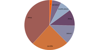](https://elm-visualization.netlify.app/PieChart/)\n\n@docs arc, Arc, centroid\n\n\n# Pies\n\n@docs PieConfig, pie, defaultPieConfig\n\n\n# Lines\n\n[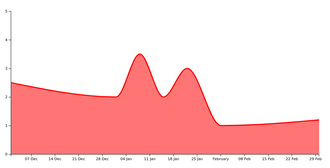](https://elm-visualization.netlify.app/LineChart/)\n\n@docs line, lineRadial, area, areaRadial\n\n\n# Curves\n\nWhile lines are defined as a sequence of two-dimensional [x, y] points, and areas are similarly\ndefined by a topline and a baseline, there remains the task of transforming this discrete representation\ninto a continuous shape: i.e., how to interpolate between the points. A variety of curves are provided for this purpose.\n\n@docs linearCurve\n@docs basisCurve, basisCurveClosed, basisCurveOpen\n@docs bumpXCurve, bumpYCurve\n@docs bundleCurve\n@docs cardinalCurve, cardinalCurveClosed, cardinalCurveOpen\n@docs catmullRomCurve, catmullRomCurveClosed, catmullRomCurveOpen\n@docs monotoneInXCurve, monotoneInYCurve\n@docs stepCurve, naturalCurve\n\n\n# Stack\n\nA stack is a way to fit multiple graphs into one drawing. Rather than drawing graphs on top of each other,\nthe layers are stacked. This is useful when the relation between the graphs is of interest.\n\nIn most cases, the absolute size of a piece of data becomes harder to determine for the reader.\n\n@docs StackConfig, StackResult, stack\n\n\n## Stack Offset\n\nThe method of stacking.\n\n@docs stackOffsetNone, stackOffsetDiverging, stackOffsetExpand, stackOffsetSilhouette, stackOffsetWiggle\n\n\n## Stack Order\n\nThe order of the layers. Normal list functions can be used, for instance\n\n -- keep order of the input data\n identity\n\n -- reverse\n List.reverse\n\n -- decreasing by sum of the values (largest is lowest)\n List.sortBy (Tuple.second >> List.sum >> negate)\n\n@docs sortByInsideOut\n\n","unions":[],"aliases":[{"name":"Arc","comment":" Used to configure an `arc`. These can be generated by a `pie`, but you can\neasily modify these later.\n\n\n### innerRadius : Float\n\nUsefull for creating a donut chart. A negative value is treated as zero. If larger\nthan `outerRadius` they are swapped.\n\n\n### outerRadius : Float\n\nThe radius of the arc. A negative value is treated as zero. If smaller\nthan `innerRadius` they are swapped.\n\n\n### cornerRadius : Float\n\nIf the corner radius is greater than zero, the corners of the arc are rounded\nusing circles of the given radius. For a circular sector, the two outer corners\nare rounded; for an annular sector, all four corners are rounded. The corner\ncircles are shown in this diagram:\n\n[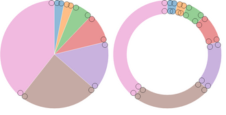](https://elm-visualization.netlify.app/CornerRadius/)\n\nThe corner radius may not be larger than `(outerRadius - innerRadius) / 2`.\nIn addition, for arcs whose angular span is less than π, the corner radius may\nbe reduced as two adjacent rounded corners intersect. This is occurs more often\nwith the inner corners.\n\n\n### startAngle : Float\n\nThe angle is specified in radians, with 0 at -y (12 o’clock) and positive angles\nproceeding clockwise. If |endAngle - startAngle| ≥ τ, a complete circle or\nannulus is generated rather than a sector.\n\n\n### endAngle : Float\n\nThe angle is specified in radians, with 0 at -y (12 o’clock) and positive angles\nproceeding clockwise. If |endAngle - startAngle| ≥ τ, a complete circle or annulus\nis generated rather than a sector.\n\n\n### padAngle : Float\n\nThe pad angle is converted to a fixed linear distance separating adjacent arcs,\ndefined as padRadius \\* padAngle. This distance is subtracted equally from the\nstart and end of the arc. If the arc forms a complete circle or annulus,\nas when |endAngle - startAngle| ≥ τ, the pad angle is ignored.\n\nIf the inner radius or angular span is small relative to the pad angle, it may\nnot be possible to maintain parallel edges between adjacent arcs. In this case,\nthe inner edge of the arc may collapse to a point, similar to a circular sector.\nFor this reason, padding is typically only applied to annular sectors\n(i.e., when innerRadius is positive), as shown in this diagram:\n\n[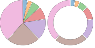](https://elm-visualization.netlify.app/PadAngle/)\n\nThe recommended minimum inner radius when using padding is outerRadius \\* padAngle / sin(θ),\nwhere θ is the angular span of the smallest arc before padding. For example,\nif the outer radius is 200 pixels and the pad angle is 0.02 radians,\na reasonable θ is 0.04 radians, and a reasonable inner radius is 100 pixels.\n\nOften, the pad angle is not set directly on the arc generator, but is instead\ncomputed by the pie generator so as to ensure that the area of padded arcs is\nproportional to their value.\nIf you apply a constant pad angle to the arc generator directly, it tends to\nsubtract disproportionately from smaller arcs, introducing distortion.\n\n\n### padRadius : Float\n\nThe pad radius determines the fixed linear distance separating adjacent arcs,\ndefined as padRadius \\* padAngle.\n\n","args":[],"type":"{ innerRadius : Basics.Float, outerRadius : Basics.Float, cornerRadius : Basics.Float, startAngle : Basics.Float, endAngle : Basics.Float, padAngle : Basics.Float, padRadius : Basics.Float }"},{"name":"PieConfig","comment":" Used to configure a `pie` generator function.\n\n`innerRadius`, `outerRadius`, `cornerRadius` and `padRadius` are simply forwarded\nto the `Arc` result. They are provided here simply for convenience.\n\n\n### valueFn : a -> Float\n\nThis is used to compute the actual numerical value used for computing the angles.\nYou may use a `List.map` to preprocess data into numbers instead, but this is\nuseful if trying to use `sortingFn`.\n\n\n### sortingFn : a -> a -> Order\n\nSorts the data. Sorting does not affect the order of the generated arc list,\nwhich is always in the same order as the input data list; it merely affects\nthe computed angles of each arc. The first arc starts at the start angle and the\nlast arc ends at the end angle.\n\n\n### startAngle : Float\n\nThe start angle here means the overall start angle of the pie, i.e., the start\nangle of the first arc. The units of angle are arbitrary, but if you plan to use\nthe pie generator in conjunction with an arc generator, you should specify an\nangle in radians, with 0 at -y (12 o’clock) and positive angles proceeding clockwise.\n\n\n### endAngle : Float\n\nThe end angle here means the overall end angle of the pie, i.e., the end angle\nof the last arc. The units of angle are arbitrary, but if you plan to use the\npie generator in conjunction with an arc generator, you should specify an angle\nin radians, with 0 at -y (12 o’clock) and positive angles proceeding clockwise.\n\nThe value of the end angle is constrained to startAngle ± τ, such that |endAngle - startAngle| ≤ τ.\n\n\n### padAngle : Float\n\nThe pad angle here means the angular separation between each adjacent arc. The\ntotal amount of padding reserved is the specified angle times the number of\nelements in the input data list, and at most |endAngle - startAngle|; the\nremaining space is then divided proportionally by value such that the relative\narea of each arc is preserved.\n\n","args":["a"],"type":"{ startAngle : Basics.Float, endAngle : Basics.Float, padAngle : Basics.Float, sortingFn : a -> a -> Basics.Order, valueFn : a -> Basics.Float, innerRadius : Basics.Float, outerRadius : Basics.Float, cornerRadius : Basics.Float, padRadius : Basics.Float }"},{"name":"StackConfig","comment":" Configuration for a stacked chart.\n\n - `data`: List of values with an accompanying label.\n - `offset`: How to stack the layers on top of each other.\n - `order`: sorting function to determine the order of the layers.\n\nSome example configs:\n\n stackedBarChart : StackConfig String\n stackedBarChart =\n { data = myData\n , offset = Shape.stackOffsetNone\n , order =\n -- stylistic choice: largest (by sum of values)\n -- category at the bottom\n List.sortBy (Tuple.second >> List.sum >> negate)\n }\n\n streamgraph : StackConfig String\n streamgraph =\n { data = myData\n , offset = Shape.stackOffsetWiggle\n , order = Shape.sortByInsideOut (Tuple.second >> List.sum)\n }\n\n","args":["a"],"type":"{ data : List.List ( a, List.List Basics.Float ), offset : List.List (List.List ( Basics.Float, Basics.Float )) -> List.List (List.List ( Basics.Float, Basics.Float )), order : List.List ( a, List.List Basics.Float ) -> List.List ( a, List.List Basics.Float ) }"},{"name":"StackResult","comment":" The basis for constructing a stacked chart\n\n - `values`: Sorted list of values, where every item is a `(yLow, yHigh)` pair.\n - `labels`: Sorted list of labels\n - `extent`: The minimum and maximum y-value. Convenient for creating scales.\n\n","args":["a"],"type":"{ values : List.List (List.List ( Basics.Float, Basics.Float )), labels : List.List a, extent : ( Basics.Float, Basics.Float ) }"}],"values":[{"name":"arc","comment":" The arc generator produces a [circular](https://en.wikipedia.org/wiki/Circular_sector)\nor [annular](https://en.wikipedia.org/wiki/Annulus_%28mathematics%29) sector, as in\na pie or donut chart. If the difference between the start and end angles (the\nangular span) is greater than [τ](https://en.wikipedia.org/wiki/Turn_%28geometry%29#Tau_proposals),\nthe arc generator will produce a complete circle or annulus. If it is less than\n[τ](https://en.wikipedia.org/wiki/Turn_%28geometry%29#Tau_proposal), arcs may have\nrounded corners and angular padding. Arcs are always centered at ⟨0,0⟩; use a\ntransform to move the arc to a different position.\n\nSee also the pie generator, which computes the necessary angles to represent an\narray of data as a pie or donut chart; these angles can then be passed to an arc\ngenerator.\n\n","type":"Shape.Arc -> Path.Path"},{"name":"area","comment":" The area generator produces an area, as in an area chart. An area is defined\nby two bounding lines, either splines or polylines. Typically, the two lines\nshare the same x-values (x0 = x1), differing only in y-value (y0 and y1);\nmost commonly, y0 is defined as a constant representing zero. The first line\n(the topline) is defined by x1 and y1 and is rendered first; the second line\n(the baseline) is defined by x0 and y0 and is rendered second, with the points\nin reverse order. With a `linearCurve` curve, this produces a clockwise polygon.\n\nThe data attribute you pass in should be a `[Just ((x0, y0), (x1, y1))]`. Passing\nin `Nothing` represents gaps in the data and corresponding gaps in the area will\nbe rendered.\n\nUsually you will need to convert your data into a format supported by this function.\nFor example, if your data is a `List (Date, Float)`, you might use something like:\n\n areaGenerator : ( Date, Float ) -> Maybe ( ( Float, Float ), ( Float, Float ) )\n areaGenerator ( x, y ) =\n Just\n ( ( Scale.convert xScale x, Tuple.first (Scale.rangeExtent yScale) )\n , ( Scale.convert xScale x, Scale.convert yScale y )\n )\n\n areaPath : List ( Date, Float ) -> Path\n areaPath data =\n List.map areaGenerator data\n |> Shape.area Shape.linearCurve\n\nwhere `xScale` and `yScale` would be appropriate `Scale`s.\n\n","type":"(List.List ( Basics.Float, Basics.Float ) -> SubPath.SubPath) -> List.List (Maybe.Maybe ( ( Basics.Float, Basics.Float ), ( Basics.Float, Basics.Float ) )) -> Path.Path"},{"name":"areaRadial","comment":" This works exactly like `area`, except it interprets the points it recieves as `(angle, radius)`\npairs, where radius is in _radians_. Therefore it renders a radial layout with a center at `(0, 0)`.\n\nUse a transform to position the layout in final rendering.\n\n","type":"(List.List ( Basics.Float, Basics.Float ) -> SubPath.SubPath) -> List.List (Maybe.Maybe ( ( Basics.Float, Basics.Float ), ( Basics.Float, Basics.Float ) )) -> Path.Path"},{"name":"basisCurve","comment":" Produces a cubic [basis spline](https://en.wikipedia.org/wiki/B-spline) using the specified control points.\nThe first and last points are triplicated such that the spline starts at the first point and ends at the last\npoint, and is tangent to the line between the first and second points, and to the line between the penultimate\nand last points.\n\n[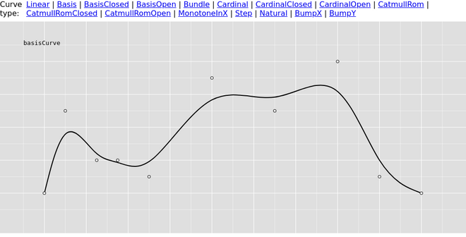](https://elm-visualization.netlify.app/Curves/#basis)\n\n","type":"List.List ( Basics.Float, Basics.Float ) -> SubPath.SubPath"},{"name":"basisCurveClosed","comment":" Produces a closed cubic basis spline using the specified control points. When a line segment ends, the first three control points are repeated, producing a closed loop with C2 continuity.\n\n[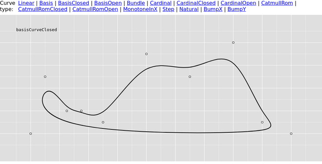](https://elm-visualization.netlify.app/Curves/#basisclosed)\n\n","type":"List.List ( Basics.Float, Basics.Float ) -> SubPath.SubPath"},{"name":"basisCurveOpen","comment":" Produces a cubic basis spline using the specified control points. Unlike basis, the first and last points are not repeated, and thus the curve typically does not intersect these points.\n\n[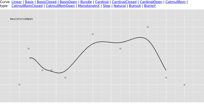](https://elm-visualization.netlify.app/Curves/#basisopen)\n\n","type":"List.List ( Basics.Float, Basics.Float ) -> SubPath.SubPath"},{"name":"bumpXCurve","comment":" Produces a Bézier curve between each pair of points, with horizontal tangents at each point.\n\n[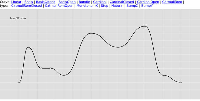](https://elm-visualization.netlify.app/Curves/#bumpx)\n\n","type":"List.List ( Basics.Float, Basics.Float ) -> SubPath.SubPath"},{"name":"bumpYCurve","comment":" Produces a Bézier curve between each pair of points, with vertical tangents at each point.\n\n[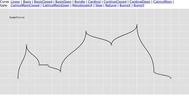](https://elm-visualization.netlify.app/Curves/#bumpy)\n\n","type":"List.List ( Basics.Float, Basics.Float ) -> SubPath.SubPath"},{"name":"bundleCurve","comment":" Produces a straightened cubic [basis spline](https://en.wikipedia.org/wiki/B-spline) using the specified control points,\nwith the spline straightened according to the curve’s beta (a reasonable default is `0.85`). This curve is typically\nused in hierarchical edge bundling to disambiguate connections, as proposed by Danny Holten\nin [Hierarchical Edge Bundles: Visualization of Adjacency Relations in Hierarchical Data](https://www.researchgate.net/profile/Danny_Holten/publication/6715561_Hierarchical_Edge_Bundles_Visualization_of_Adjacency_Relations_in_Hierarchical_Data/links/0deec535a57c5dc79d000000/Hierarchical-Edge-Bundles-Visualization-of-Adjacency-Relations-in-Hierarchical-Data.pdf?origin=publication_detail).\n\nThis curve is not suitable to be used with areas.\n\n[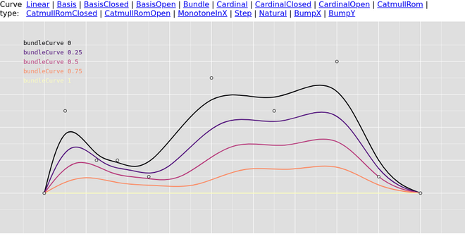](https://elm-visualization.netlify.app/Curves/#bundle)\n\n","type":"Basics.Float -> List.List ( Basics.Float, Basics.Float ) -> SubPath.SubPath"},{"name":"cardinalCurve","comment":" Produces a cubic [cardinal spline](https://en.wikipedia.org/wiki/Cubic_Hermite_spline#Cardinal_spline) using\nthe specified control points, with one-sided differences used for the first and last piece.\n\nThe tension parameter determines the length of the tangents: a tension of one yields all zero tangents, equivalent to\n`linearCurve`; a tension of zero produces a uniform Catmull–Rom spline.\n\n[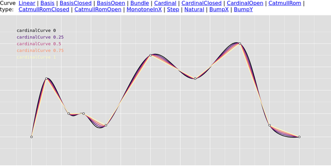](https://elm-visualization.netlify.app/Curves/#cardinal)\n\n","type":"Basics.Float -> List.List ( Basics.Float, Basics.Float ) -> SubPath.SubPath"},{"name":"cardinalCurveClosed","comment":" Produces a cubic [cardinal spline](https://en.wikipedia.org/wiki/Cubic_Hermite_spline#Cardinal_spline) using\nthe specified control points. At the end, the first three control points are repeated, producing a closed loop.\n\nThe tension parameter determines the length of the tangents: a tension of one yields all zero tangents, equivalent to\n`linearCurve`; a tension of zero produces a uniform Catmull–Rom spline.\n\n[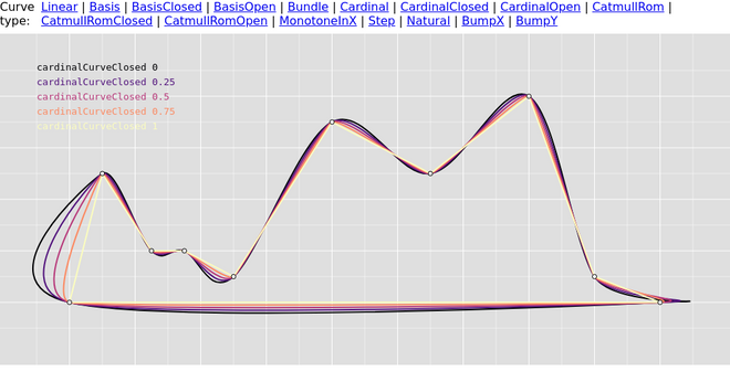](https://elm-visualization.netlify.app/Curves/#cardinalclosed)\n\n","type":"Basics.Float -> List.List ( Basics.Float, Basics.Float ) -> SubPath.SubPath"},{"name":"cardinalCurveOpen","comment":" Produces a cubic [cardinal spline](https://en.wikipedia.org/wiki/Cubic_Hermite_spline#Cardinal_spline) using\nthe specified control points. Unlike curveCardinal, one-sided differences are not used for the first and last piece, and thus the curve starts at the second point and ends at the penultimate point.\n\nThe tension parameter determines the length of the tangents: a tension of one yields all zero tangents, equivalent to\n`linearCurve`; a tension of zero produces a uniform Catmull–Rom spline.\n\n[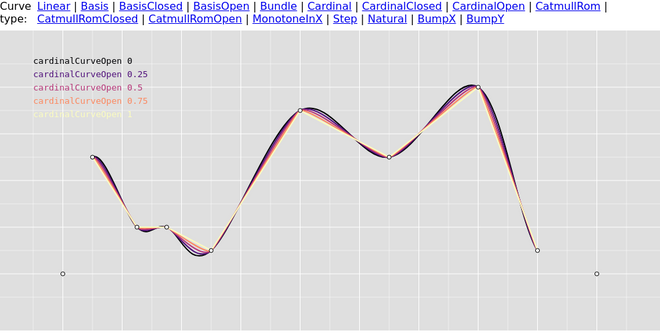](https://elm-visualization.netlify.app/Curves/#cardinalopen)\n\n","type":"Basics.Float -> List.List ( Basics.Float, Basics.Float ) -> SubPath.SubPath"},{"name":"catmullRomCurve","comment":" Produces a cubic Catmull–Rom spline using the specified control points and the parameter alpha (a good default is 0.5),\nas proposed by Yuksel et al. in [On the Parameterization of Catmull–Rom Curves](http://www.cemyuksel.com/research/catmullrom_param/),\nwith one-sided differences used for the first and last piece.\n\nIf alpha is zero, produces a uniform spline, equivalent to `curveCardinal` with a tension of zero; if alpha is one,\nproduces a chordal spline; if alpha is 0.5, produces a [centripetal spline](https://en.wikipedia.org/wiki/Centripetal_Catmull–Rom_spline).\nCentripetal splines are recommended to avoid self-intersections and overshoot.\n\n[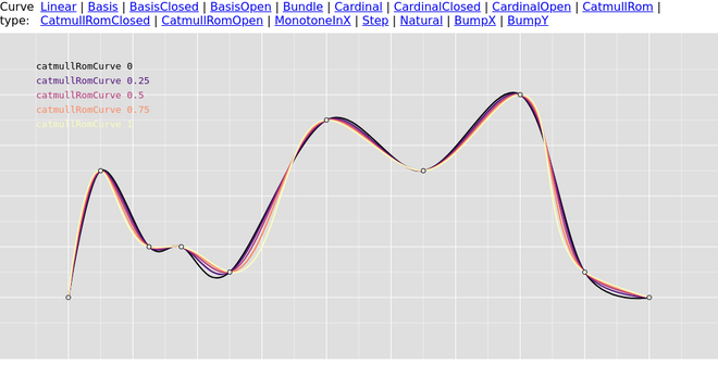](https://elm-visualization.netlify.app/Curves/#catmullrom)\n\n","type":"Basics.Float -> List.List ( Basics.Float, Basics.Float ) -> SubPath.SubPath"},{"name":"catmullRomCurveClosed","comment":" Produces a cubic Catmull–Rom spline using the specified control points and the parameter alpha (a good default is 0.5),\nas proposed by Yuksel et al. When a line segment ends, the first three control points are repeated, producing a closed loop.\n\nIf alpha is zero, produces a uniform spline, equivalent to `curveCardinal` with a tension of zero; if alpha is one,\nproduces a chordal spline; if alpha is 0.5, produces a [centripetal spline](https://en.wikipedia.org/wiki/Centripetal_Catmull–Rom_spline).\nCentripetal splines are recommended to avoid self-intersections and overshoot.\n\n[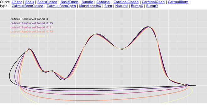](https://elm-visualization.netlify.app/Curves/#catmullromclosed)\n\n","type":"Basics.Float -> List.List ( Basics.Float, Basics.Float ) -> SubPath.SubPath"},{"name":"catmullRomCurveOpen","comment":" Produces a cubic Catmull–Rom spline using the specified control points and the parameter alpha (a good default is 0.5),\nas proposed by Yuksel et al. Unlike curveCatmullRom, one-sided differences are not used for the first and last piece, and thus the curve starts at the second point and ends at the penultimate point.\n\nIf alpha is zero, produces a uniform spline, equivalent to `curveCardinal` with a tension of zero; if alpha is one,\nproduces a chordal spline; if alpha is 0.5, produces a [centripetal spline](https://en.wikipedia.org/wiki/Centripetal_Catmull–Rom_spline).\nCentripetal splines are recommended to avoid self-intersections and overshoot.\n\n[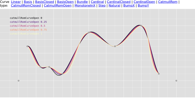](https://elm-visualization.netlify.app/Curves/#catmullromopen)\n\n","type":"Basics.Float -> List.List ( Basics.Float, Basics.Float ) -> SubPath.SubPath"},{"name":"centroid","comment":" Computes the midpoint (x, y) of the center line of the arc that would be\ngenerated by the given arguments. The midpoint is defined as\n(startAngle + endAngle) / 2 and (innerRadius + outerRadius) / 2. For example:\n\n[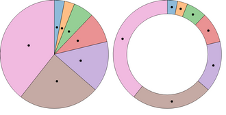](https://elm-visualization.netlify.app/Centroid/)\n\nNote that this is not the geometric center of the arc, which may be outside the arc;\nthis function is merely a convenience for positioning labels.\n\n","type":"Shape.Arc -> ( Basics.Float, Basics.Float )"},{"name":"defaultPieConfig","comment":" The default config for generating pies.\n\n import Shape exposing (defaultPieConfig)\n\n pieData =\n Shape.pie { defaultPieConfig | outerRadius = 230 } model\n\nNote that if you change `valueFn`, you will likely also want to change `sortingFn`.\n\n","type":"Shape.PieConfig Basics.Float"},{"name":"line","comment":" Generates a line for the given array of points which can be passed to the `d`\nattribute of the `path` SVG element. It needs to be suplied with a curve function.\nPoints accepted are `Maybe`s, Nothing represent gaps in the data and corresponding\ngaps will be rendered in the line.\n\n**Note:** A single point (surrounded by Nothing) may not be visible.\n\nUsually you will need to convert your data into a format supported by this function.\nFor example, if your data is a `List (Date, Float)`, you might use something like:\n\n lineGenerator : ( Date, Float ) -> Maybe ( Float, Float )\n lineGenerator ( x, y ) =\n Just ( Scale.convert xScale x, Scale.convert yScale y )\n\n linePath : List ( Date, Float ) -> Path\n linePath data =\n List.map lineGenerator data\n |> Shape.line Shape.linearCurve\n\nwhere `xScale` and `yScale` would be appropriate `Scale`s.\n\n","type":"(List.List ( Basics.Float, Basics.Float ) -> SubPath.SubPath) -> List.List (Maybe.Maybe ( Basics.Float, Basics.Float )) -> Path.Path"},{"name":"lineRadial","comment":" This works exactly like `line`, except it interprets the points it recieves as `(angle, radius)`\npairs, where radius is in _radians_. Therefore it renders a radial layout with a center at `(0, 0)`.\n\nUse a transform to position the layout in final rendering.\n\n","type":"(List.List ( Basics.Float, Basics.Float ) -> SubPath.SubPath) -> List.List (Maybe.Maybe ( Basics.Float, Basics.Float )) -> Path.Path"},{"name":"linearCurve","comment":" Produces a polyline through the specified points.\n\n[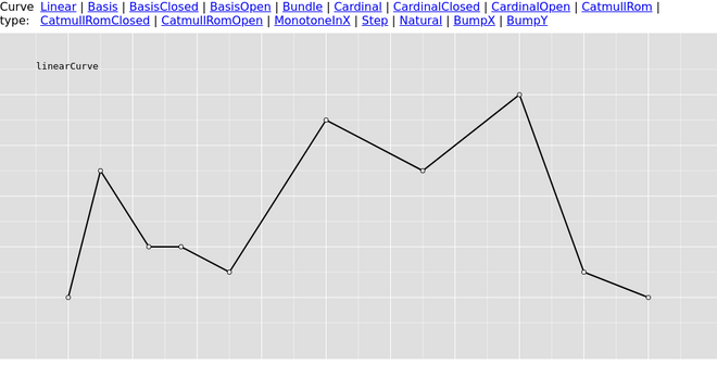](https://elm-visualization.netlify.app/Curves/#linear)\n\n","type":"List.List ( Basics.Float, Basics.Float ) -> SubPath.SubPath"},{"name":"monotoneInXCurve","comment":" Produces a cubic spline that [preserves monotonicity](https://en.wikipedia.org/wiki/Monotonic_function)\nin y, assuming monotonicity in x, as proposed by Steffen in\n[A simple method for monotonic interpolation in one dimension](http://adsabs.harvard.edu/full/1990A%26A...239..443S):\n“a smooth curve with continuous first-order derivatives that passes through any\ngiven set of data points without spurious oscillations. Local extrema can occur\nonly at grid points where they are given by the data, but not in between two adjacent grid points.”\n\n[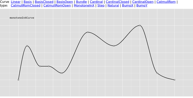](https://elm-visualization.netlify.app/Curves/#monotoneinx)\n\n","type":"List.List ( Basics.Float, Basics.Float ) -> SubPath.SubPath"},{"name":"monotoneInYCurve","comment":" Produces a cubic spline that [preserves monotonicity](https://en.wikipedia.org/wiki/Monotonic_function)\nin y, assuming monotonicity in y, as proposed by Steffen in\n[A simple method for monotonic interpolation in one dimension](http://adsabs.harvard.edu/full/1990A%26A...239..443S):\n“a smooth curve with continuous first-order derivatives that passes through any\ngiven set of data points without spurious oscillations. Local extrema can occur\nonly at grid points where they are given by the data, but not in between two adjacent grid points.”\n","type":"List.List ( Basics.Float, Basics.Float ) -> SubPath.SubPath"},{"name":"naturalCurve","comment":" Produces a [natural](https://en.wikipedia.org/wiki/Spline_interpolation) [cubic spline](http://mathworld.wolfram.com/CubicSpline.html)\nwith the second derivative of the spline set to zero at the endpoints.\n\n[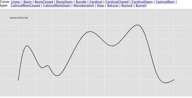](https://elm-visualization.netlify.app/Curves/#natural)\n\n","type":"List.List ( Basics.Float, Basics.Float ) -> SubPath.SubPath"},{"name":"pie","comment":" The pie generator does not produce a shape directly, but instead computes\nthe necessary angles to represent a tabular dataset as a pie or donut chart;\nthese angles can then be passed to an `arc` generator.\n","type":"Shape.PieConfig a -> List.List a -> List.List Shape.Arc"},{"name":"sortByInsideOut","comment":" Sort such that small values are at the outer edges, and large values in the middle.\n\nThis is the recommended order for stream graphs.\n\n","type":"(a -> Basics.Float) -> List.List a -> List.List a"},{"name":"stack","comment":" Create a stack result\n","type":"Shape.StackConfig a -> Shape.StackResult a"},{"name":"stackOffsetDiverging","comment":" \n\nPositive values are stacked above zero, negative values below zero.\n\n stackOffsetDiverging [ [ (0, 42) ], [ (0, -24) ] ]\n --> [ [ (0, 42) ], [ (-24, 0 ) ] ]\n\n stackOffsetDiverging [ [ (0, 42), (0, -20) ], [ (0, -24), (0, -24) ] ]\n --> [[(0,42),(-20,0)],[(-24,0),(-44,-20)]]\n\n","type":"List.List (List.List ( Basics.Float, Basics.Float )) -> List.List (List.List ( Basics.Float, Basics.Float ))"},{"name":"stackOffsetExpand","comment":" \n\nApplies a zero baseline and normalizes the values for each point such that the topline is always one.\n\n stackOffsetExpand [ [ (0, 50) ], [ (50, 100) ] ]\n --> [[(0,0.5)],[(0.5,1)]]\n\n","type":"List.List (List.List ( Basics.Float, Basics.Float )) -> List.List (List.List ( Basics.Float, Basics.Float ))"},{"name":"stackOffsetNone","comment":" \n\nStacks the values on top of each other, starting at 0.\n\n stackOffsetNone [ [ (0, 42) ], [ (0, 70) ] ]\n --> [ [ (0, 42) ], [ (42, 112 ) ] ]\n\n stackOffsetNone [ [ (0, 42) ], [ (20, 70) ] ]\n --> [ [ (0, 42) ], [ (42, 112 ) ] ]\n\n","type":"List.List (List.List ( Basics.Float, Basics.Float )) -> List.List (List.List ( Basics.Float, Basics.Float ))"},{"name":"stackOffsetSilhouette","comment":" \n\nShifts the baseline down such that the center of the streamgraph is always at zero.\n\n stackOffsetSilhouette [ [ (0, 50) ], [ (50, 100) ] ]\n --> [[(-75,-25)],[(-25,75)]]\n\n","type":"List.List (List.List ( Basics.Float, Basics.Float )) -> List.List (List.List ( Basics.Float, Basics.Float ))"},{"name":"stackOffsetWiggle","comment":" \n\nShifts the baseline so as to minimize the weighted wiggle of layers.\n\nVisually, high wiggle means peaks going in both directions very close to each other. The silhouette stack offset above often suffers\nfrom having high wiggle.\n\n stackOffsetWiggle [ [ (0, 50) ], [ (50, 100) ] ]\n --> [[(0,50)],[(50,150)]]\n\n","type":"List.List (List.List ( Basics.Float, Basics.Float )) -> List.List (List.List ( Basics.Float, Basics.Float ))"},{"name":"stepCurve","comment":" Produces a piecewise constant function (a step function) consisting of alternating horizontal and vertical lines.\n\nThe factor parameter changes when the y-value changes between each pair of adjacent x-values.\n\n[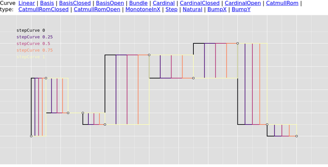](https://elm-visualization.netlify.app/Curves/#step)\n\n","type":"Basics.Float -> List.List ( Basics.Float, Basics.Float ) -> SubPath.SubPath"}],"binops":[]},{"name":"Statistics","comment":"\n\n@docs extent, extentBy, extentWith\n\n@docs variance, deviation, quantile\n\n@docs peaks\n\n\n# Transformations\n\nMethods for transforming list and for generating new lists.\n\n@docs ticks, tickStep, range\n\n","unions":[],"aliases":[],"values":[{"name":"deviation","comment":" Returns the standard deviation, defined as the square root of the [bias-corrected variance](#variance), of the given\nlist of numbers. If the list has fewer than two values, returns Nothing.\n","type":"List.List Basics.Float -> Maybe.Maybe Basics.Float"},{"name":"extent","comment":" Returns the minimum and maximum value in the list.\n","type":"List.List comparable -> Maybe.Maybe ( comparable, comparable )"},{"name":"extentBy","comment":" Returns the minimum and maximum value in the given array using comparisons\nfrom values passed by the accessor function.\n\n data : List { name : String, age : Int}\n data =\n [ {name = \"John Smith\", age = 32 }\n , {name = \"Mark Luther\", age = 45 }\n , {name = \"Cory Jones\", age = 26 }\n ]\n\n extentBy .age data\n --> Just ({name = \"Cory Jones\", age = 26 }\n --> , {name = \"Mark Luther\", age = 45 })\n\n","type":"(a -> comparable) -> List.List a -> Maybe.Maybe ( a, a )"},{"name":"extentWith","comment":" Returns the minimum and maximum value in the given array using comparisons\nprovided by the comparison function.\n","type":"(a -> a -> Basics.Order) -> List.List a -> Maybe.Maybe ( a, a )"},{"name":"peaks","comment":" This functions detects (positive) peaks in a timeseries.\n\nThe first argument is there to extract the actual value to perform the computation on.\n\nIt also accepts some parameters to tune the behavior of the function:\n\n - `lookaround`: Each value will be compared to this many neigbours on both sides and will get a score on how much taller it is then the shortest of them.\n\n - `sensitivity`: This is used as a threshold to filter the candidate peaks to select the gloably biggest.\n\n - `coallesce`: To prevent peaks that span multiple samples, this parameter will coalesce these into a single sample.\n\n peaks identity { lookaround = 2, sensitivity = 1.4, coallesce = 0 } [ 2, 0, 10, 2, 1 ] --> [ 10 ]\n\nBased on work by [Yuri Vishnevsky](https://observablehq.com/@yurivish/peak-detection).\n\n","type":"(a -> Basics.Float) -> { lookaround : Basics.Int, sensitivity : Basics.Float, coallesce : Basics.Int } -> List.List a -> List.List a"},{"name":"quantile","comment":" Returns the p-quantile of the given **sorted** list of numbers, where `p` is a number in the range [0, 1]. For\nexample, the median can be computed using p = 0.5, the first quartile at p = 0.25, and the third quartile at p = 0.75.\nThis particular implementation uses the [R-7 method](https://en.wikipedia.org/wiki/Quantile#Quantiles_of_a_population),\nwhich is the default for the R programming language and Excel. For example:\n\n a : List Float\n a = [0, 10, 30]\n\n quantile 0 a --> Just 0\n quantile 0.5 a --> Just 10\n quantile 1 a --> Just 30\n quantile 0.25 a --> Just 5\n quantile 0.75 a --> Just 20\n quantile 0.1 a --> Just 2\n\n","type":"Basics.Float -> List.List Basics.Float -> Maybe.Maybe Basics.Float"},{"name":"range","comment":" Returns a List containing an arithmetic progression, similar to the Python\nbuilt-in range. This method is often used to iterate over a sequence of\nuniformly-spaced numeric values, such as the indexes of an array or the ticks of\na linear scale. (See also [ticks](#ticks) for nicely-rounded values.)\n\nTakes a `start`, `stop` and `step` argument. The stop value is exclusive; it is not\nincluded in the result. If `step` is positive, the last element is the largest\n`start + i * step` less than `stop`; if `step` is negative, the last element is\nthe smallest `start + i * step` greater than `stop`. If the returned list would\ncontain an infinite number of values, an empty range is returned.\n\nThe arguments are not required to be whole numbers; however, the results are more\npredictable if they are.\n\nDifferences from [List.range from the standard library](https://package.elm-lang.org/packages/elm/core/latest/List#range):\n\n - `List.range` is inclusive, meaning that the stop value will be included in the result\n - `List.range` supports `Int`, whereas this uses `Float`\n - `List.range` supports only increasing intervals (i.e. `List.range 3 1 == []` vs. `range 3 1 -1 == [3, 2]`)\n - `List.range` doesn't allow for specifying the step value\n\n","type":"Basics.Float -> Basics.Float -> Basics.Float -> List.List Basics.Float"},{"name":"tickStep","comment":" Returns the difference between adjacent tick values if the same arguments\nwere passed to `ticks`: a nicely-rounded value that is a power of ten multiplied\nby 1, 2 or 5. Note that due to the limited precision of IEEE 754 floating point,\nthe returned value may not be exact decimals.\n\n tickStep 1.9 6.4 10 -- 0.5\n\n tickStep 1.9 6 5 -- 1\n\n","type":"Basics.Float -> Basics.Float -> Basics.Int -> Basics.Float"},{"name":"ticks","comment":" Returns a list of approximately n + 1 uniformly-spaced, nicely-rounded\nvalues between a start and stop value (inclusive). Each value is a power of ten\nmultiplied by 1, 2 or 5. Note that due to the limited precision of IEEE 754\nfloating point, the returned values may not be exact decimals.\n\nTicks are inclusive in the sense that they may include the specified start and\nstop values if (and only if) they are exact, nicely-rounded values consistent\nwith the inferred step. More formally, each returned tick t satisfies\nstart ≤ t and t ≤ stop.\n\n ticks 1.9 6.4 10 --> [2, 2.5, 3, 3.5, 4, 4.5, 5, 5.5, 6]\n\n ticks 1.9 6 5 --> [2, 3, 4, 5, 6]\n\n","type":"Basics.Float -> Basics.Float -> Basics.Int -> List.List Basics.Float"},{"name":"variance","comment":" Returns an [unbiased estimator of the population variance](http://mathworld.wolfram.com/SampleVariance.html) of the\ngiven list of numbers. If the list has fewer than two values, returns Nothing.\n","type":"List.List Basics.Float -> Maybe.Maybe Basics.Float"}],"binops":[]},{"name":"Transition","comment":" Transition is a module for writing animations. It does not attempt to be an animation library for every use case,\nit is specifically designed for the needs of data visualization apps. The main idea is that one animates data in some\nintermediate form and then leaves the `view` function to display the data as normal.\n\n\n### Setting up animation in an app\n\nWhile there are many ways to use this module, a typical setup will look like this:\n\n import Browser.Events\n import Interpolation exposing (Interpolator)\n import Transition exposing (Transition)\n\n type alias Model =\n { transition : Transition MyThing\n }\n\n type Msg\n = Tick Int\n | StartAnimation MyThing\n\nFirst setup a default transition that doesn't actually do anything:\n\n init : () -> ( Model, Cmd Msg )\n init () =\n ( { transition = Transition.constant initialThing }\n , Cmd.none\n )\n\nNext setup a subscription:\n\n subscriptions : Model -> Sub Msg\n subscriptions model =\n if Transition.isComplete model.transition then\n Sub.none\n\n else\n Browser.Events.onAnimationFrameDelta (round >> Tick)\n\nDefine an interpolator for your value:\n\n interpolateThing : MyThing -> MyThing -> Interpolator MyThing\n interpolateThing from to =\n -- ...\n\nThen handle stuff in your update function:\n\n update : Msg -> Model -> ( Model, Cmd Msg )\n update msg model =\n case msg of\n Tick t ->\n ( { model\n | transition = Transition.step t model.transition\n }\n , Cmd.none\n )\n\n StartAnimation newThing ->\n let\n oldThing =\n Transition.value model.transition\n in\n ( { model\n | transition =\n Transition.for 600 (interpolateThing oldThing newThing)\n }\n , Cmd.none\n )\n\nThen make your view like normal:\n\n view : Model -> Html Msg\n view model =\n viewMyThing (Transition.value model.transition)\n\n viewMyThing : MyThing -> Html Msg\n viewMyThing thing =\n --- ...\n\n\n## Transitions\n\n@docs Transition, for, easeFor, constant, step, value, isComplete, reverse\n\n\n## Repetition\n\n@docs repeat, repeatAlternate, repeatIndefinitely, repeatAlternateIndefinitely\n\n\n## Staggered animation\n\n@docs stagger\n\n\n## Easing\n\n@docs Easing, easeLinear, easeCubic, easePolynomialIn, easePolynomialOut, easePolynomial, easeSinusoidalIn, easeSinusoidalOut, easeSinusoidal, easeExponentialIn, easeExponentialOut, easeExponential, easeCircleIn, easeCircleOut, easeCircle, easeElasticIn, easeElasticOut, easeElastic, easeBackIn, easeBackOut, easeBack, easeBounceIn, easeBounceOut, easeBounce\n\n","unions":[{"name":"Easing","comment":" Easing is a method of distorting time to control apparent motion in animation. It is most commonly used for [slow-in, slow-out](https://en.wikipedia.org/wiki/Twelve_basic_principles_of_animation#Slow_In_and_Slow_Out). By easing time, animated transitions are smoother and exhibit more plausible motion.\n","args":[],"cases":[]},{"name":"Transition","comment":" A transition is a smooth interpolation between a beginning state and an end state, with a duration and easing.\n","args":["a"],"cases":[]}],"aliases":[],"values":[{"name":"constant","comment":" A transition that is already complete that will always return the value passed in.\n","type":"a -> Transition.Transition a"},{"name":"easeBack","comment":" Symmetric anticipatory easing.\n","type":"Basics.Float -> Transition.Easing"},{"name":"easeBackIn","comment":" [Anticipatory](https://en.wikipedia.org/wiki/Twelve_basic_principles_of_animation#Anticipation) easing, like a dancer bending his knees before jumping off the floor. The degree of overshoot is configurable. A reasonable default is 1.70158. [This represents about 10% more than the difference between the numbers](http://void.heteml.jp/blog/archives/2014/05/easing_magicnumber.html).\n","type":"Basics.Float -> Transition.Easing"},{"name":"easeBackOut","comment":" Reverse anticipatory easing.\n","type":"Basics.Float -> Transition.Easing"},{"name":"easeBounce","comment":" Symmetric bounce easing.\n","type":"Transition.Easing"},{"name":"easeBounceIn","comment":" Bounce easing, like a rubber ball.\n","type":"Transition.Easing"},{"name":"easeBounceOut","comment":" Reverse bounce easing.\n","type":"Transition.Easing"},{"name":"easeCircle","comment":" Symetric circular easing.\n","type":"Transition.Easing"},{"name":"easeCircleIn","comment":" Circular easing.\n","type":"Transition.Easing"},{"name":"easeCircleOut","comment":" Reverse circular easing.\n","type":"Transition.Easing"},{"name":"easeCubic","comment":" Symetric cubic easing. This is quite a good default for a lot of animation. Equivalent to `easePolynomial 3`\n","type":"Transition.Easing"},{"name":"easeElastic","comment":" Symmetric elastic easing.\n","type":"{ amplitude : Basics.Float, period : Basics.Float } -> Transition.Easing"},{"name":"easeElasticIn","comment":" Elastic easing, like a rubber band. Reasonable defaults for the parameters would be `{ amplitude = 1, period = 0.3 }`.\n","type":"{ amplitude : Basics.Float, period : Basics.Float } -> Transition.Easing"},{"name":"easeElasticOut","comment":" Reverse elastic easing.\n","type":"{ amplitude : Basics.Float, period : Basics.Float } -> Transition.Easing"},{"name":"easeExponential","comment":" Symetric exponential easing.\n","type":"Transition.Easing"},{"name":"easeExponentialIn","comment":" Exponential easing; raises 2 to the exponent 10 \\* (t - 1).\n","type":"Transition.Easing"},{"name":"easeExponentialOut","comment":" Reverse exponential easing.\n","type":"Transition.Easing"},{"name":"easeFor","comment":" This is like `Transition.for`, but allows one to specify a custom Easing function. `Transition.for` defaults to `Transition.easeCubic`.\n","type":"Basics.Int -> Transition.Easing -> Interpolation.Interpolator a -> Transition.Transition a"},{"name":"easeLinear","comment":" Linear easing is esentially the identity function of easing.\n","type":"Transition.Easing"},{"name":"easePolynomial","comment":" Symmetric polynomial easing. In _t_ [0, 0.5] equivalent to `easePolynomialIn` in [0.5, 1] `easePolynomialOut`\n","type":"Basics.Float -> Transition.Easing"},{"name":"easePolynomialIn","comment":" Polynomial easing; raises _t_ to the provided exponent.\n","type":"Basics.Float -> Transition.Easing"},{"name":"easePolynomialOut","comment":" Reverse polynomial easing; equivalent to `1 - easePolynomialIn (1 - t)`.\n","type":"Basics.Float -> Transition.Easing"},{"name":"easeSinusoidal","comment":" Symmetric sinusoidal easing\n","type":"Transition.Easing"},{"name":"easeSinusoidalIn","comment":" Sinusoidal easing; returns sin(t).\n","type":"Transition.Easing"},{"name":"easeSinusoidalOut","comment":" Reverse sinusoidal easing; equivalent to 1 - sinIn(1 - t).\n","type":"Transition.Easing"},{"name":"for","comment":" Create a transition that will run _for_ a certain number of miliseconds. You need to provide an interpolation between the start and end states.\n\nFor example to fade something in for 400ms:\n\n fadeIn : Item -> Transition Item\n fadeIn item =\n Interpolation.map (\\opacity -> { item | opacity = opacity)\n (Interpolation.float 0 1)\n |> Transition.for 400\n\n","type":"Basics.Int -> Interpolation.Interpolator a -> Transition.Transition a"},{"name":"isComplete","comment":" Allows you to check if a transition has finished running. This can be used to clean up subscriptions.\n","type":"Transition.Transition a -> Basics.Bool"},{"name":"repeat","comment":" Repeat the transition a number of times.\n","type":"Basics.Int -> Transition.Transition a -> Transition.Transition a"},{"name":"repeatAlternate","comment":" Repeat the transition a set number of times, but run every even run in reverse.\n","type":"Basics.Int -> Transition.Transition a -> Transition.Transition a"},{"name":"repeatAlternateIndefinitely","comment":" Keep running the transition indefinitely, but alternating forward and reverse runs.\n","type":"Transition.Transition a -> Transition.Transition a"},{"name":"repeatIndefinitely","comment":" Keep running the transition.\n","type":"Transition.Transition a -> Transition.Transition a"},{"name":"reverse","comment":" Reverses the direction of a transition running it backwards.\n","type":"Transition.Transition a -> Transition.Transition a"},{"name":"stagger","comment":" Run a bunch of animations with a duration and easing, but delay each successive animation by the delay amount.\n\n**Tip:** You may find the `List (Interpolator a) -> Transition (List a)` a little inconvenient for organizing staggered animations.\nHowever, you can create an `List (Interpolator (a -> a))`, where each function touches and interpolates some orthogonal property,\nthen `List.foldl (\\fn val -> fn val) model.target (Transition.value model.transition)`. This way you can stagger updates to almost any\ndatastructure. However, you need to be somewhat careful if there are other ways the datastructure can be changed (like user input) to\nmake sure to interupt the animation suitably.\n\n type Foo =\n { position: (Float, Float)\n , color : Color\n }\n\n [ \\t foo -> { foo | position = interpolatePosition t }\n , \\t foo -> { foo | color = Interpolation.rgb Color.blue Color.red t }\n ]\n |> Transition.stagger { durationEach = 200, delay = 100, easing Transition.easingCubic }\n\nWill first start animating the position, then after 100ms start animating the color, for a total duration of 300ms.\n\n","type":"{ durationEach : Basics.Int, delay : Basics.Int, easing : Transition.Easing } -> List.List (Interpolation.Interpolator a) -> Transition.Transition (List.List a)"},{"name":"step","comment":" Updates the internal state forward by the passed number of miliseconds. You would typically do this in your `update` function.\n","type":"Basics.Int -> Transition.Transition a -> Transition.Transition a"},{"name":"value","comment":" Returns the \"current\" value. You would typically call this in the view and render whatever this returns.\n\n import Interpolation\n\n transition : Transition Int\n transition =\n Transition.easeFor 500 Transition.easeLinear (Interpolation.int 0 10)\n\n transition |> Transition.value --> 0\n transition |> Transition.step 250 |> Transition.value --> 5\n transition |> Transition.step 600 |> Transition.value --> 10\n\n","type":"Transition.Transition a -> a"}],"binops":[]},{"name":"Zoom","comment":" This module implements a convenient abstraction for panning and zooming:\nit lets the user focus on a regions of interest in a visualization.\nIt is quite intuitive in that dragging the mouse coresponds to panning,\nmouse wheel zooming, and touch interactions are also supported.\n\nThe implementation is agnostic about the DOM, so it can be used with HTML, SVG, or WebGL.\n\n\n## Setting up zooming in your app\n\nWhile there are many ways to use this module, a typical setup will look like this:\n\n import Zoom exposing (OnZoom, Zoom)\n\n type alias Model =\n { zoom : Zoom\n }\n\n type Msg\n = ZoomMsg OnZoom\n\n -- ...\n\nNext, initialize and configure the zoom model:\n\n init : () -> ( Model, Cmd Msg )\n init () =\n ( { zoom = Zoom.init { width = width, height = height } }\n , Cmd.none\n )\n\nNote that you will need to provide the width and height of the element that you want to setup the zooming behavior for. If you don't know this information, then you might want to use [`Browser.Dom.getElement`](https://package.elm-lang.org/packages/elm/browser/latest/Browser-Dom#getElement) to get it.\n\nNext setup a subscription:\n\n subscriptions : Model -> Sub Msg\n subscriptions model =\n Zoom.subscriptions model.zoom ZoomMsg\n\nThen handle update:\n\n update : Msg -> Model -> ( Model, Cmd Msg )\n update msg model =\n case msg of\n ZoomMsg zoomMsg ->\n ( { model\n | zoom = Zoom.update zoomMsg model.zoom\n }\n , Cmd.none\n )\n\nFinally, set up your view:\n\n view : Model -> Html Msg\n view model =\n svg\n (A.width width\n :: A.height height\n :: Zoom.transform model.zoom\n :: Zoom.events model.zoom ZoomMsg\n )\n [ myChildrenElements ]\n\n\n## Configuring the zoom behavior\n\n@docs Zoom, init, scaleExtent, translateExtent\n\n\n## Updating the zoom\n\n@docs OnZoom, update, subscriptions\n\n\n## Manipulating the zoom transform programmatically\n\n@docs setTransform, TransitionOption, instantly, animatedAround\n\n\n## View\n\n@docs transform, asRecord\n\n\n## Handling User Events\n\n@docs events, onDoubleClick, onWheel, onDrag, onGesture, onTouch\n\n","unions":[{"name":"OnZoom","comment":" This is the Msg type used. You will want to pass these to `Zoom.update`.\n\nNote that when handling these messages, it is also extremely likely that the zoom transform has somehow changed,\nso you can also use that place in your update function to react to that. For example in a map application, you may\nwant to fetch a different tile based on the zoom level:\n\n update : Msg -> Model -> ( Model, Cmd Msg )\n update msg model =\n case msg of\n Zoomed onZoom ->\n let\n oldTransform =\n Zoom.asRecord model.zoom\n\n newZoom =\n Zoom.update onZoom model.zoom\n\n newTransform =\n Zoom.asRecord newZoom\n\n cmd =\n if toTileCoords oldTransform /= toTileCoords newTransform then\n fetchTile (toTileCoords newTransform)\n\n else\n Cmd.none\n in\n ( { model | zoom = newZoom }, cmd )\n\n","args":[],"cases":[]},{"name":"TransitionOption","comment":" Enumerates the ways a zoom transform can be changed.\n","args":[],"cases":[]},{"name":"Zoom","comment":" This type will go into your model as it stores the internal state and configuration necessary to support the various user interactions.\n","args":[],"cases":[]}],"aliases":[],"values":[{"name":"animatedAround","comment":" Animates the zoom transform minimizing movement around the specified point.\n","type":"( Basics.Float, Basics.Float ) -> Zoom.TransitionOption"},{"name":"asRecord","comment":" Returns the actual transform for the view relative to the top left corner. You can then use these numbers to transform the view as necessary.\n","type":"Zoom.Zoom -> { scale : Basics.Float, translate : { x : Basics.Float, y : Basics.Float } }"},{"name":"events","comment":" Sets up the event handlers necessary to support this behavior on various devices.\n\nIt is merely a convenience, implemented such:\n\n events zoom tagger =\n Zoom.onDoubleClick zoom tagger\n :: Zoom.onWheel zoom tagger\n :: Zoom.onDrag zoom tagger\n ++ Zoom.onGesture zoom tagger\n ++ Zoom.onTouch zoom tagger\n\nSo if you want to customize the user experience, you can for example omit the onWheel handler in your own defintion.\n\n","type":"Zoom.Zoom -> (Zoom.OnZoom -> msg) -> List.List (Svg.Attribute msg)"},{"name":"init","comment":" Creates a brand new `Zoom`. You have to pass in the dimensions (in pixels) of the element that you want to make zoom-eable.\n","type":"{ width : Basics.Float, height : Basics.Float } -> Zoom.Zoom"},{"name":"instantly","comment":" Changes the zoom transform instantly.\n","type":"Zoom.TransitionOption"},{"name":"onDoubleClick","comment":" Zooms in on double click, zooms out on double click while holding shift.\n","type":"Zoom.Zoom -> (Zoom.OnZoom -> msg) -> Svg.Attribute msg"},{"name":"onDrag","comment":" Allows panning on mouse drag.\n","type":"Zoom.Zoom -> (Zoom.OnZoom -> msg) -> List.List (Svg.Attribute msg)"},{"name":"onGesture","comment":" Supports pinch to zoom on desktop Safari.\n","type":"Zoom.Zoom -> (Zoom.OnZoom -> msg) -> List.List (Svg.Attribute msg)"},{"name":"onTouch","comment":" Supports pinch to zoom on mobile devices.\n","type":"Zoom.Zoom -> (Zoom.OnZoom -> msg) -> List.List (Svg.Attribute msg)"},{"name":"onWheel","comment":" Zooms on mousewheel.\n","type":"Zoom.Zoom -> (Zoom.OnZoom -> msg) -> Svg.Attribute msg"},{"name":"scaleExtent","comment":" Allows you to set a minimum and maximum scale that the user will be able to zoom to.\n\nTypically there is only limited resolution to the data, so setting the maximum such that the maximum resolution is comfortably visible (remember accessibility - some people will want to zoom a fair bit more than you might find necessary) would be a good idea.\n\nThe miminum zoom will always be asymptotically approaching zero, but setting a higher number is good, because the view can be \"lost\" if it gets too small. Typically you would set it such that the whole dataset fits into the view.\n\n","type":"Basics.Float -> Basics.Float -> Zoom.Zoom -> Zoom.Zoom"},{"name":"setTransform","comment":" Change the zoom transform programmatically.\n","type":"Zoom.TransitionOption -> { scale : Basics.Float, translate : { x : Basics.Float, y : Basics.Float } } -> Zoom.Zoom -> Zoom.Zoom"},{"name":"subscriptions","comment":" Subrscriptions are used for allowing drags to continue outside the element as well for animated zooms on double-click.\n","type":"Zoom.Zoom -> (Zoom.OnZoom -> msg) -> Platform.Sub.Sub msg"},{"name":"transform","comment":" A convenience for setting up the `tranform` attribute for **SVG** elements.\n","type":"Zoom.Zoom -> Svg.Attribute msg"},{"name":"translateExtent","comment":" Allows you to set a boundary where a user will be able to pan to. The format is `((left, top), (right, bottom))`.\n\nTypically you will want to set this to `((0, 0), (width, height))`, however you can restrict it however you like. For example maps typically only restrict vertical movement, but not horizontal movement.\n\n","type":"( ( Basics.Float, Basics.Float ), ( Basics.Float, Basics.Float ) ) -> Zoom.Zoom -> Zoom.Zoom"},{"name":"update","comment":" This is what you need to set up in your update function.\n","type":"Zoom.OnZoom -> Zoom.Zoom -> Zoom.Zoom"}],"binops":[]}]