This repository has been archived by the owner on Apr 28, 2023. It is now read-only.
-
Notifications
You must be signed in to change notification settings - Fork 0
/
Copy path01_data_in_R.Rmd
233 lines (119 loc) · 16.2 KB
/
01_data_in_R.Rmd
1
2
3
4
5
6
7
8
9
10
11
12
13
14
15
16
17
18
19
20
21
22
23
24
25
26
27
28
29
30
31
32
33
34
35
36
37
38
39
40
41
42
43
44
45
46
47
48
49
50
51
52
53
54
55
56
57
58
59
60
61
62
63
64
65
66
67
68
69
70
71
72
73
74
75
76
77
78
79
80
81
82
83
84
85
86
87
88
89
90
91
92
93
94
95
96
97
98
99
100
101
102
103
104
105
106
107
108
109
110
111
112
113
114
115
116
117
118
119
120
121
122
123
124
125
126
127
128
129
130
131
132
133
134
135
136
137
138
139
140
141
142
143
144
145
146
147
148
149
150
151
152
153
154
155
156
157
158
159
160
161
162
163
164
165
166
167
168
169
170
171
172
173
174
175
176
177
178
179
180
181
182
183
184
185
186
187
188
189
190
191
192
193
194
195
196
197
198
199
200
201
202
203
204
205
206
207
208
209
210
211
212
213
214
215
216
217
218
219
220
221
222
223
224
225
226
227
228
229
230
231
232
233
# Data in R
You've already been working with data throughout this set of courses. You've generated your own data in Google Sheets (i.e. collected data from Leanpub). You've worked with datasets that are included in RStudio automatically (i.e. `iris` and `mtcars`). And, you've generated R Markdown documents and pushed code to GitHub, creating even more data! But, we haven't formalized exactly what all the different types of data are in R, how to access them, and what the various file types in R are. We'll discuss all of that in this lesson.
Then, throughout the following lessons in this course, you'll learn how to work with data in R. Specifically, you'll learn how to get data into a usable format for data analysis. This process is called **data wrangling**, and we'll use datasets available to you from R and RStudio to learn the necessary tools for you to excel at data wrangling.
Finally, to give you an idea of where we're going, once you have a set of skills down to functionally work with data, in the next course in this series you'll learn about lots of different places where you can get data and how to get them into R, so you can continue to practice the data wrangling skills you'll learn here!
### File Types in R
In previous lessons we talked about R Markdown documents (which have the file extension .rmd or .Rmd) and we've saved R script files (which have the file extension .r or .R), but we haven't formally discussed what all the various types of files are used for in detail or about what other possible file types exist in R. So, we'll do that now!
Before discussing further details about each type of file, we'll point out that the file extension (what comes after the period in the file name) specifies what type of file you're working with. While the extension matters (.R is different than .Rmd), capitalization does not matter for file extensions (.r is the same as .R). Just something to keep in mind as you start working with these types of files.
That said, while the *computer* will know what type of file it is regardless of capitalization, when you're writing code, capitalization *does* matter. If you try to read in a file named "script.r" but accidentally specify "script.R", your code won't be able to find the file. We mention this now so as you start saving files you save files using consistent capitalization). The capitalization in each of the sections below is the capitalization we recommend. We'll summarize this here before walking through each one. For following file extensions, we recommend the following capitalization:
* Scripting files: .R
* R Markdown: .Rmd
* Saved R Objects: .rda
* Serialized R Objects: .rds
* R Project files .Rproj
#### R Script file (.R)
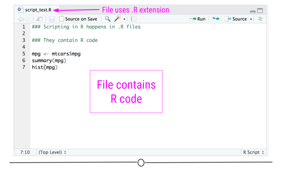
The most basic file type in R uses the .R file extension. R Script files contain code written in the R programming language. As you want to write R code and save this code, you'll save it as a .R file.
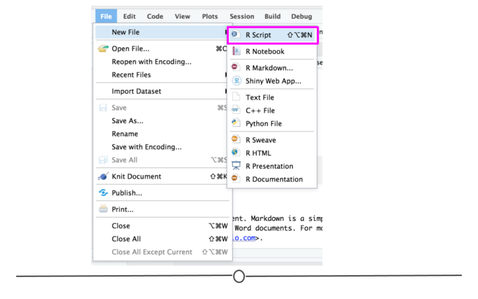
To get started writing an R Script file, you'll go to [rstudio.cloud](rstudio.cloud) and click on File > New File > RScript along the menu at the top. This will open ups a blank R Script file.
In this R Script is where you would write R code. As you write code, you'll want to save this file. Here, in this example, you can see the R code we've written and that this file has been saved as "script_test.R."
#### R Markdown (.Rmd)
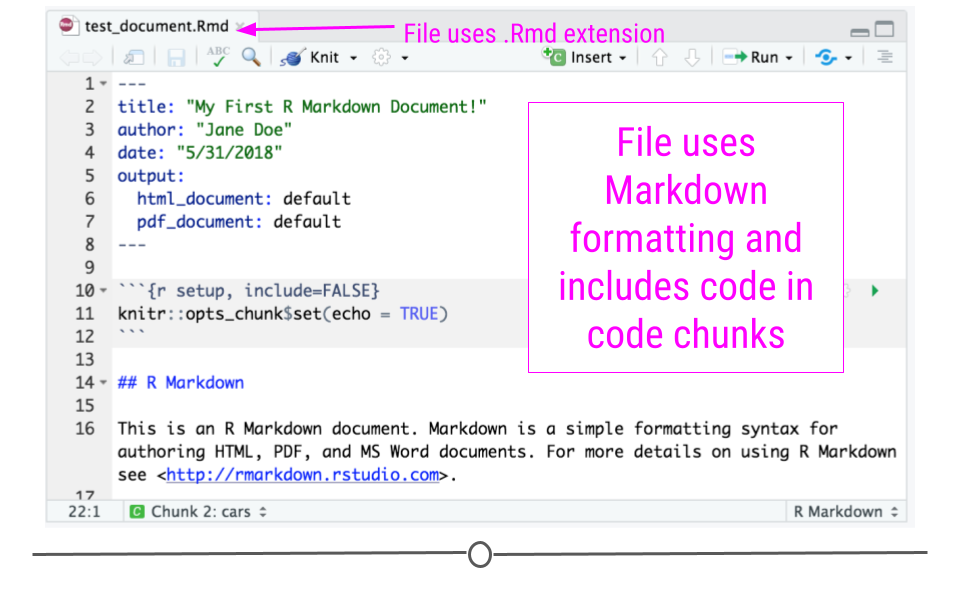
We've also introduced R Markdown files previously. As a refresher, R Markdown documents use Markdown syntax *and* include code chunks with R code that will be run when the document is "Knit" into its final format (which can be PDF, HTML, or Word documents among others.
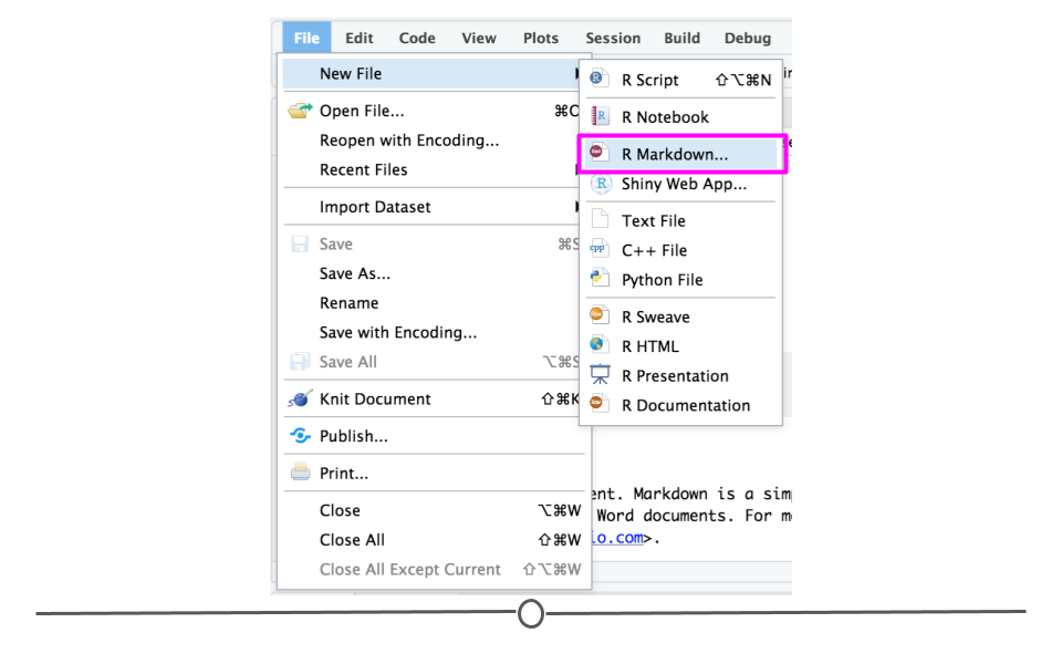
To get started writing an R Markdown document, you'll go to [rstudio.cloud](rstudio.cloud) and click on File > New File > R Markdown... After filling out the information in the pop-up window and clicking OK, an R Markdown document will open up.
In this document you'll use Markdown syntax outside of code chunks and R code in the code chunks to generate your reports.
R Markdown documents are great at producing reproducible reports that walk people through your data science process from start to finish.
#### Saved R objects (.rda, .RData)
As you write R code (say, in an .R file), you will inevitably create objects. For example, in the code you see here, `mpg` is an object created by this code that contains the data from the `mpg` column of the `mtcars` data frame and `cyl` an object from the `cyl` column of the `mtcars` data frame.
```r
mpg <- mtcars$mpg
cyl <- mtcars$cyl
```
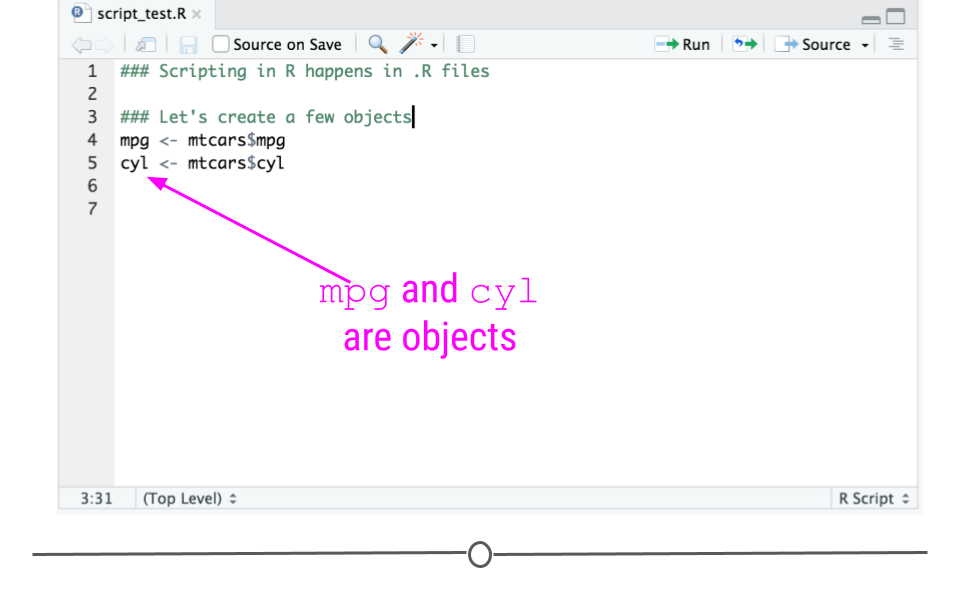
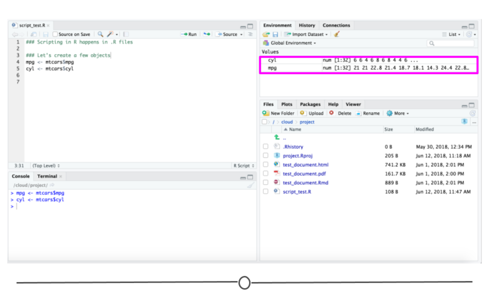
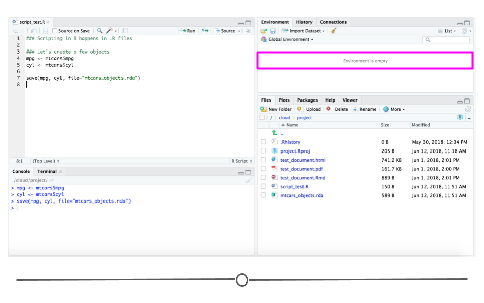
If I were to run these two lines of code, they would show up in the Console, and the objects `mpg` and `cyl` would now be visible in the Environment tab.
Often you'll create objects that you won't need to save. However, from time to time you'll make changes to a data frame or generate an object that you'll want to use later. To save an object and use it later, you can save it as an R data file. These files contain objects that can be saved directly *from* and read directly *into* R using the commands `save()` and `load()`. And, in particular, R data files can **save multiple objects**.
To save the two objects `mpg` and `cyl` into an R Data file, you would do the following:
```r
save(mpg, cyl, file="mtcars_objects.rda")
```
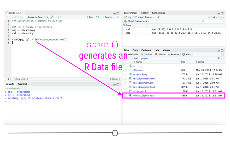
The syntax for `save` requires you to specify the objects you want to save, separated by commas. Then, the filename you want this R data file to have is specified using the `file=` argument. When this line of code is run, the specified file (here, `mtcars_objects.rda`) appears in the Files tab within RStudio, demonstrating that this file has been created.
If in the future, if you were to want to load the objects `mpg` and `cyl` back into your R session, you would do this using `load()`. To do that here, we'll first have to remove these objects from RStudio. To accomplish this, click on the broom in the Environment tab of RStudio Cloud.
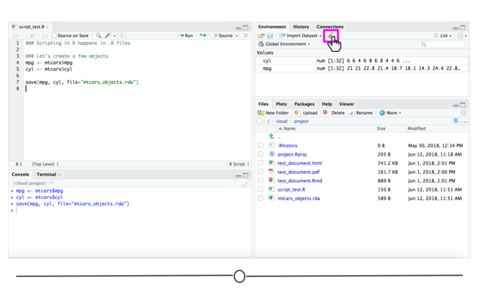
After clicking "Yes" to confirm that you want to remove all objects, you'll see that `mpg` and `cyl` are no longer in your RStudio environment. They have been removed from RStudio.
To load them back in from `mtcars_objects.rda`, you would do the following:
```r
load("mtcars_objects.rda")
```
Note that you need to put quotes around the filename to specify that this is a file and *not* an object in R.
A second note is a reminder about file paths. Here, the file we want is in the directory we're working in. If that were not the case, you would have to specify the path to the file within the quotation marks (i.e. "path/to/file/mtcars_objects.rda")
When you run this line of code, you'll see that `cyl` and `mpg` are once again available objects in your RStudio Environment tab!
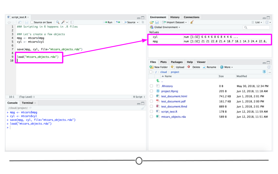
To recap, when you want to save multiple objects to be read in at a later time, you'll save them as an R data file (.rda). R Data files are generated using the `save()` function and read into R using the `load()` command.
#### Serialized R objects (.rds)
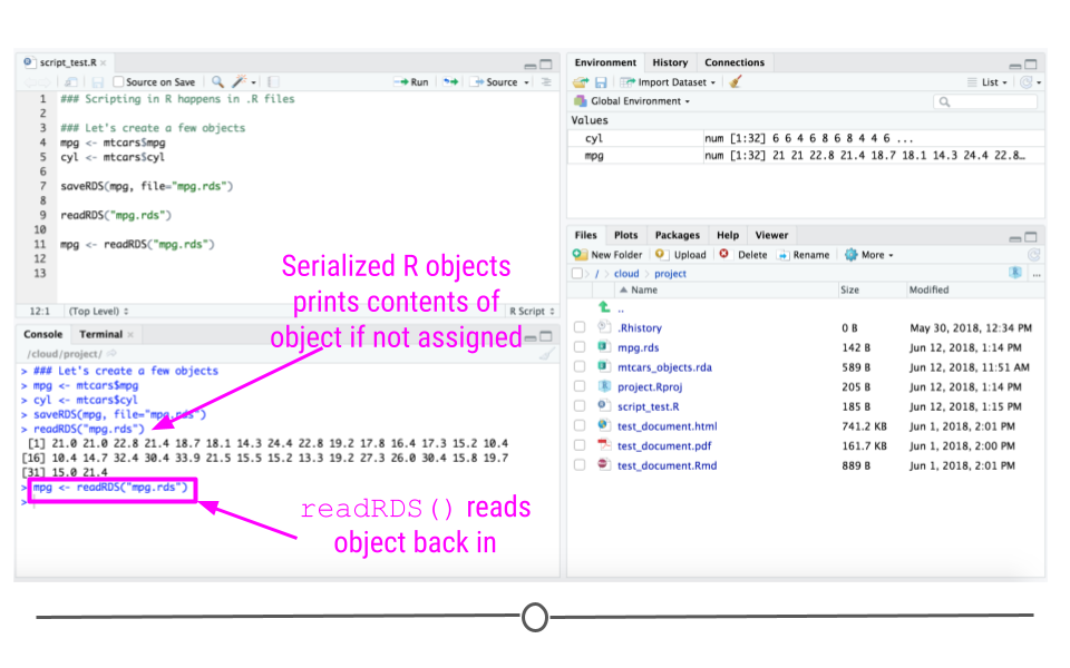
Serialized R object files are similar to R data files with the exception that they can only save a *single* R object at a time. When you only want to save a single object (say, `mpg`), these files are the best option.
To save a serialized R object file, you'll use the function `saveRDS()`. To read a serialized object file into R, you'll use the function `readRDS()`.
For example, to save the `mpg` object you would use the following:
```r
saveRDS(mpg, file="mpg.rds")
```
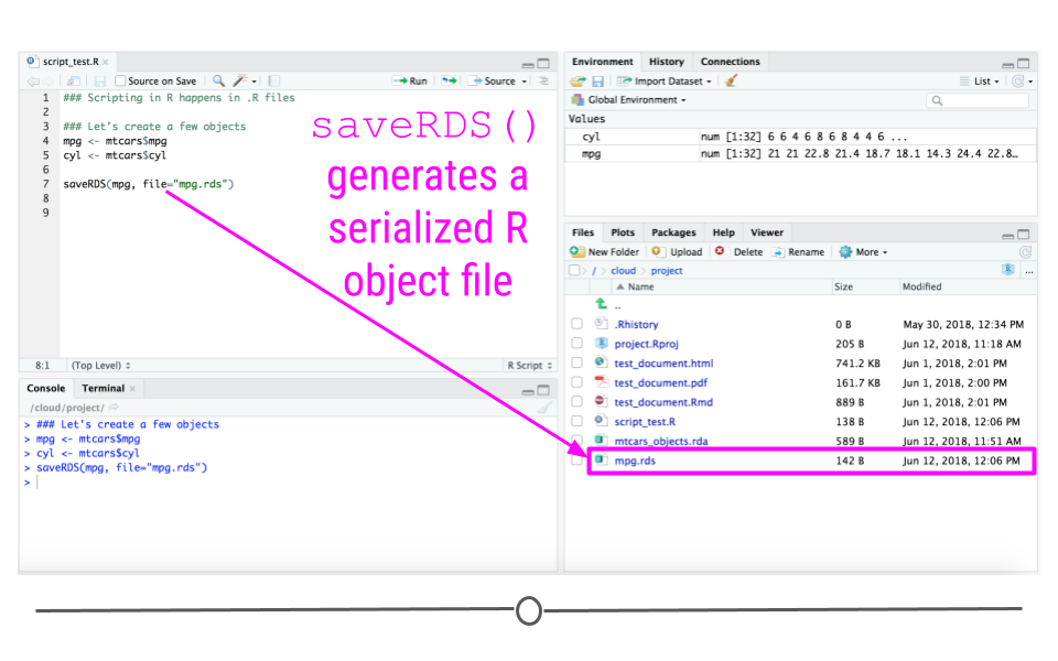
This will generate the file `mpg.rds`.
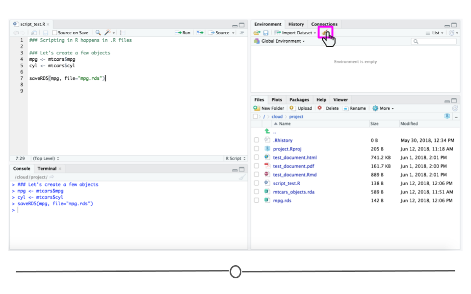
To read this file back in, we'll first remove all objects from R Studio using the broom icon in the Environment tab and will then use the `readRDS()` function.
Unlike with .rda objects, when you read a .rds object back in, to make the object available, you have to assign the object a variable name. Otherwise, the contents of the object will just print to your Console. This is helpful because it doesn't matter what the name of the object was when you saved it. As long as you know the filename, you can pick a new object name. Here, we assign the serialized R object file to `mpg`, but we could have chosen a different object name.
```r
mpg <- readRDS("mpg.rds")
```
#### R Project files (.Rproj)
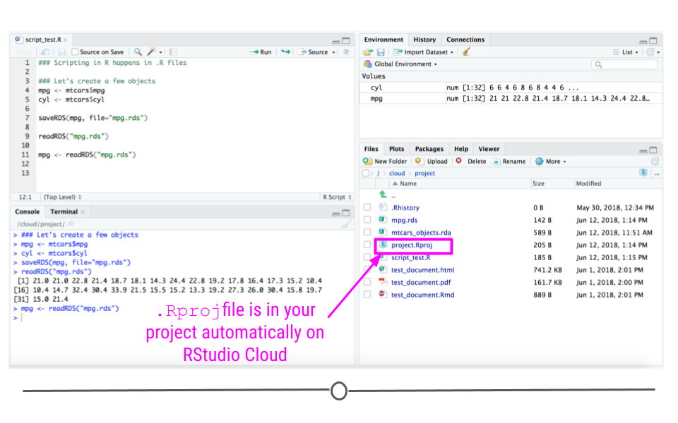
R Projects are incredibly helpful files. In their simplest form, by working within an R Project and saving an .Rproj file, you are always able to pick back up on a project from where you left off. Fortunately, RStudio Cloud uses R projects automatically. You may have noticed that there is a "project.Rproj" file in your Files tab. This is an R Project file.
RStudio Cloud will start a "project.Rproj" file within each project you start. This file will then track your project as you write code and create objects.
Then, when you return to this project, your .Rroj file will:
* start a new R session
* load the .RData file in your project's main directory file if there is one (this is the same directory where your .Rproj file is)
* load the .Rhistory file into the RStudio History tab
* set the current working directory to the project directory.
* make previously edited documents available in the Files tab
* restore RStudio settings to what they were the last time the project was closed.
This allows you to pick back up from where you left off!
Then, when you leave to work on a different project, your .RData will be saved and your .Rproj file updated so that you can pick up from where you left off the next time you sign in!
### Datasets in R
Now that we've covered the main types of R files you'll be working with and generating in RStudio, we'll move on to formally discussing the datasets available within R and RStudio/RStudio Cloud.
You've previously seen and worked with datasets that are available to you in R. Specifically, you've seen examples that used the `iris` and `mtcars` datasets in previous lessons. However, we haven't covered how to find all available datasets that are included in R automatically, so we'll do that now.
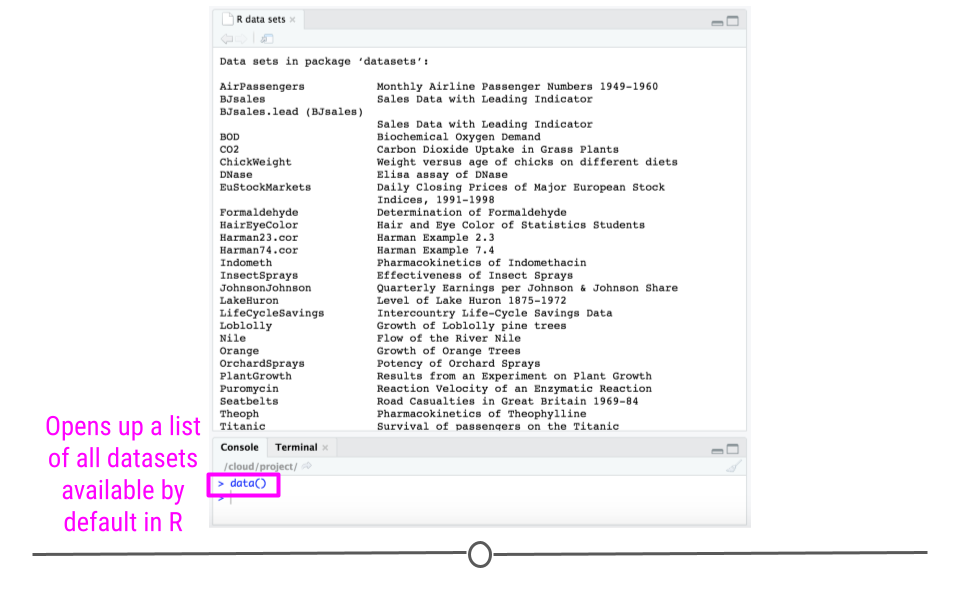
To access a list of all the available datasets within R, you'll type `data()` into your Console. This will open up a file called "R data sets". You can scroll through this list to get a sense of what data sets are available. The name of the data set is in the first column while a brief description of the dataset is in the second column.
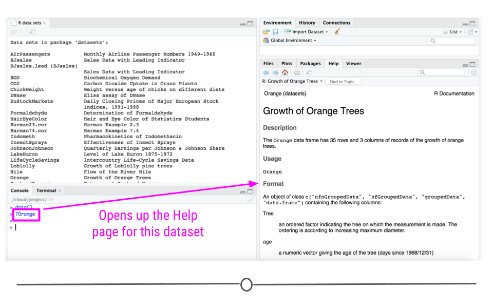
If one of these datasets looks interesting to you, say the "Orange" dataset, you can get more detailed information about the dataset by using help function in R (`?`).
```r
?Orange
```
This opens up an explanation in the Help tab of RStudio Cloud. Here, you can see a description of the dataset and can scroll to see what variables are included in this dataset. Finally, at the bottom of the Help window, you'll see examples of how to work with the dataset!
### Datasets in Packages
In addition to the datasets available by default to you in R, many packages (but not all!) also contain datasets that you can use. To see a list of what datasets are available from a specific package, you can again use the `data()` function, but you'll want to specify the name of the package using the `package=` argument
For example, to see a list of the datasets available from the ggplot2 package, you would want to use the following:
```r
data(package="ggplot2")
```
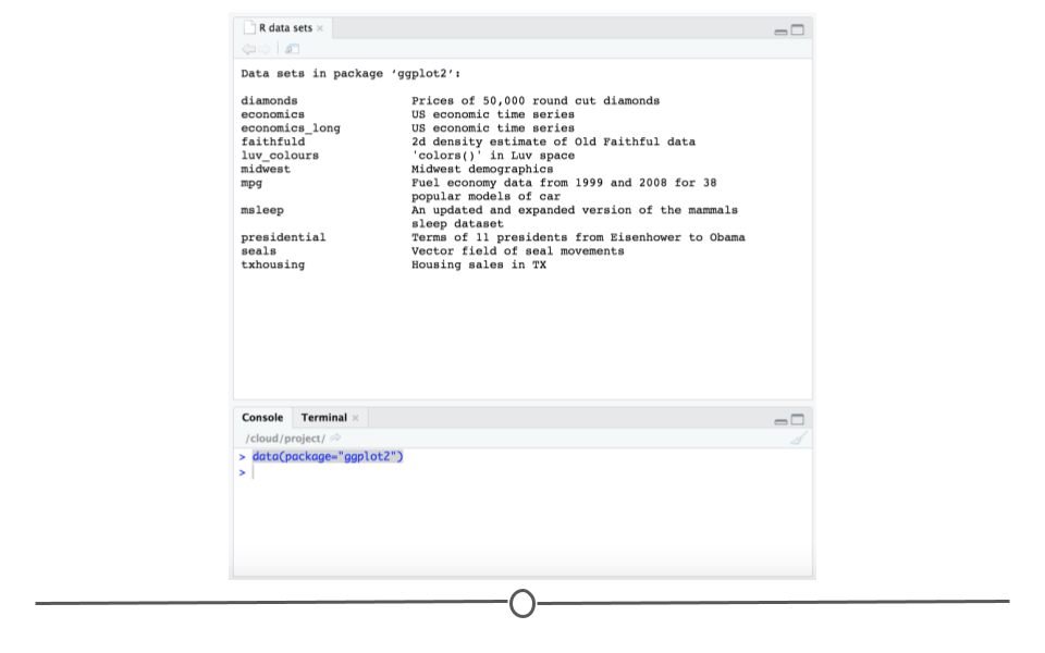
As before, this function will open up a list of the available datasets within that package.
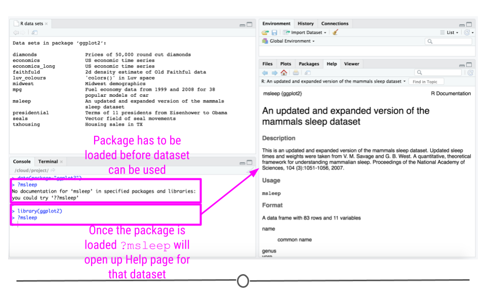
In order to use any of these datasets, however, you'll have to load the package using the `library()` function. After loading the package, you can then access the Help pages for a dataset as previously using `?`.
```r
library(ggplot2)
?msleep
```
### Other types of data in R
In addition to datasets included automatically in R/RStudio and those that are in R packages, there are lots of other types of data that can be read into R. This could be data from a Google Sheet or an Excel spreadsheet or data from a website. In the lessons in the *next* course we'll discuss a number of other types of files and master how to get them into R, so just know that's coming up! For the remaining lessons in *this* course, however, we'll stick to using datasets included in R and those included in specific R packages.
### Summary
In this lesson we've covered the main file formats that are used within R. Make sure you're comfortable with what the various file extensions mean and in what scenarios you would use the different file extensions. Additionally, we discussed how to access datasets that are available by default in RStudio as well as those that are available through specific R packages. You already have so much data at you fingertips, and we're just getting started!
### Additional Resources
* [R Studio Projects](https://support.rstudio.com/hc/en-us/articles/200526207-Using-Projects)
* [R Data files](https://thepracticalr.wordpress.com/2017/04/27/load-save-and-rda-files/)
### Slides and Video
[Automated Video](https://youtu.be/fPt9faKdhP8)
* [Slides](https://docs.google.com/presentation/d/1w7qP4LXwMUv-9mJQZgRdOqMCuUL82z7-rUGk4EoydDg/edit?usp=sharing)