Python特征选择(全)

[aialgorithm]

1 特征选择的目的

机器学习中特征选择是一个重要步骤，以筛选出显著特征、摒弃非显著特征。这样做的作用是:

• 减少特征（避免维度灾难），提高训练速度，降低运算开销；
• 减少干扰噪声，降低过拟合风险，提升模型效果；
• 更少的特征，模型可解释性更好；

2 特征选择方法

特征选择方法一般分为三类：

2.1 过滤法--特征选择

通过计算特征的缺失率、发散性、相关性、信息量、稳定性等指标对各个特征进行评估选择，常用如缺失情况、单值率、方差验证、pearson相关系数、chi2卡方检验、IV值、信息增益及PSI等方法。

2.1.1 缺失率

通过分析各特征缺失率，并设定阈值对特征进行筛选。阈值可以凭经验值（如缺失率<0.9）或可观察样本各特征整体分布，确定特征分布的异常值作为阈值。

# 特征缺失率
miss_rate_df = df.isnull().sum().sort_values(ascending=False) / df.shape[0]

2.1.2 发散性

特征无发散性意味着该特征值基本一样，无区分能力。通过分析特征单个值得最大占比及方差以评估特征发散性情况，并设定阈值对特征进行筛选。阈值可以凭经验值（如单值率<0.9, 方差>0.001）或可观察样本各特征整体分布，以特征分布的异常值作为阈值。

# 分析方差 
var_features = df.var().sort_values()
 
# 特征单值率
sigle_rate = {}
for var in df.columns:
    sigle_rate[var]=(df[var].value_counts().max()/df.shape[0])

2.1.2 相关性

特征间相关性高会浪费计算资源，影响模型的解释性。特别对线性模型来说，会导致拟合模型参数的不稳定。常用的分析特征相关性方法如：

• 方差膨胀因子VIF：

方差膨胀因子也称为方差膨胀系数（Variance Inflation），用于计算数值特征间的共线性，一般当VIF大于10表示有较高共线性。

from statsmodels.stats.outliers_influence import variance_inflation_factor
# 截距项
df['c'] = 1
name = df.columns
x = np.matrix(df)
VIF_list = [variance_inflation_factor(x,i) for i in range(x.shape[1])]
VIF = pd.DataFrame({'feature':name,"VIF":VIF_list})

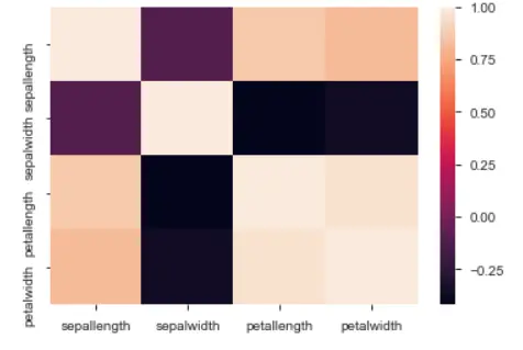
• person相关系数：
  

用于计算数值特征两两间的相关性，数值范围[-1，1]。

import seaborn as sns
corr_df=df.corr()
# 热力图
sns.heatmap(corr_df)
# 剔除相关性系数高于threshold的corr_drop
threshold = 0.9
upper = corr_df.where(np.triu(np.ones(corr_df.shape), k=1).astype(np.bool))
corr_drop = [column for column in upper.columns if any(upper[column].abs() > threshold)]

• Chi2检验

经典的卡方检验是检验类别型变量对类别型变量的相关性。

Sklearn的实现是通过矩阵相乘快速得出所有特征的观测值和期望值，在计算出各特征的 χ2 值后排序进行选择。在扩大了 chi2 的在连续型变量适用范围的同时，也方便了特征选择。

from sklearn.datasets import load_iris
from sklearn.feature_selection import SelectKBest
from sklearn.feature_selection import chi2
x, y = load_iris(return_X_y=True)

x_new = SelectKBest(chi2, k=2).fit_transform(x, y)

2.1.3 信息量

分类任务中，可以通过计算某个特征对于分类这样的事件到底有多大信息量贡献，然后特征选择信息量贡献大的特征。 常用的方法有计算IV值、信息增益。

• 信息增益

如目标变量D的信息熵为 H(D)，而D在特征A条件下的条件熵为 H(D|A)，那么信息增益 G(D , A) 为：

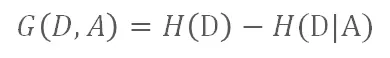
信息增益(互信息)的大小即代表特征A的信息贡献程度。

from sklearn.feature_selection import mutual_info_classif
from sklearn.datasets import load_iris
x, y = load_iris(return_X_y=True)
mutual_info_classif(x,y)

• IV

IV值(Information Value)，在风控领域是一个重要的信息量指标，衡量了某个特征（连续型变量需要先离散化）对目标变量的影响程度。其基本思想是根据该特征所命中黑白样本的比率与总黑白样本的比率，来对比和计算其关联程度。【Github代码链接】

2.1.4 稳定性

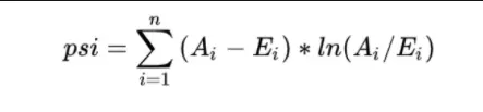
对大部分数据挖掘场景，特别是风控领域，很关注特征分布的稳定性，其直接影响到模型使用周期的稳定性。常用的是PSI（Population Stability Index，群体稳定性指标）。

• PSI

PSI表示的是实际与预期分布的差异，SUM( (实际占比 - 预期占比）* ln(实际占比 / 预期占比) )。

在建模时通常以训练样本（In the Sample, INS）作为预期分布，而验证样本作为实际分布。验证样本一般包括样本外（Out of Sample，OOS）和跨时间样本（Out of Time，OOT）【Github代码链接】

2.2 嵌入法--特征选择

嵌入法是直接使用模型训练的到特征重要性，在模型训练同时进行特征选择。通过模型得到各个特征的权值系数，根据权值系数从大到小来选择特征。常用如基于L1正则项的逻辑回归、Lighgbm特征重要性选择特征。

• 基于L1正则项的逻辑回归

L1正则方法具有稀疏解的特性，直观从二维解空间来看L1-ball 为正方形，在顶点处时(如W2=C, W1=0的稀疏解)，更容易达到最优解。可见基于L1正则方法的会趋向于产生少量的特征，而其他的特征都为0。

from sklearn.feature_selection import SelectFromModel
from sklearn.linear_model import LogisticRegression

x_new = SelectFromModel(LogisticRegression(penalty="l1", C=0.1)).fit_transform(x,  y)

• 基于树模型的特征排序

基于决策树的树模型(随机森林，Lightgbm，Xgboost等)，树生长过程中也是启发式搜索特征子集的过程，可以直接用训练后模型来输出特征重要性。

import matplotlib.pyplot as plt
from lightgbm import plot_importance
from lightgbm import LGBMClassifier


model = LGBMClassifier()
model.fit(x, y)
plot_importance(model,  max_num_features=20, figsize=(10,5),importance_type='split')
plt.show()
feature_importance = pd.DataFrame({
        'feature': model.booster_.feature_name(),
        'gain': model.booster_.feature_importance('gain'),
        'split': model.booster_.feature_importance('split')
    }).sort_values('gain',ascending=False)

当特征数量多时，对于输出的特征重要性，通常可以按照重要性的拐点划定下阈值选择特征。

2.3 包装法--特征选择

包装法是通过每次选择部分特征迭代训练模型，根据模型预测效果评分选择特征的去留。一般包括产生过程，评价函数，停止准则，验证过程，这4个部分。

(1) 产生过程( Generation Procedure )是搜索特征子集的过程，首先从特征全集中产生出一个特征子集。搜索方式有完全搜索(如广度优先搜索、定向搜索)、启发式搜索(如双向搜索、后向选择)、随机搜索(如随机子集选择、模拟退火、遗传算法)。
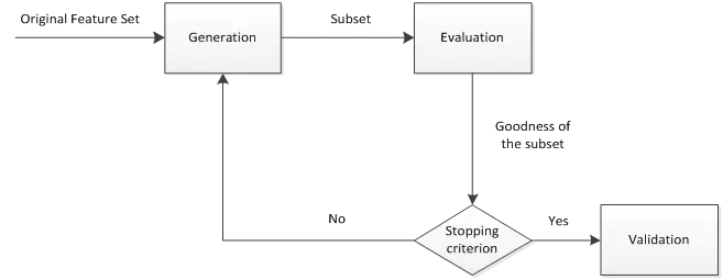
(2) 评价函数( Evaluation Function ) 是评价一个特征子集好坏程度的一个准则。
(3) 停止准则( Stopping Criterion )停止准则是与评价函数相关的，一般是一个阈值，当评价函数值达到这个阈值后就可停止搜索。
(4) 验证过程( Validation Procedure )是在验证数据集上验证选出来的特征子集的实际效果。

首先从特征全集中产生出一个特征子集，然后用评价函数对该特征子集进行评价，评价的结果与停止准则进行比较，若评价结果比停止准则好就停止，否则就继续产生下一组特征子集，继续进行特征选择。最后选出来的特征子集一般还要验证其实际效果。

• RFE

RFE递归特征消除是常见的特征选择方法。原理是递归地在剩余的特征上构建模型，使用模型判断各特征的贡献并排序后做特征选择。

from sklearn.feature_selection import RFE
rfe = RFE(estimator,n_features_to_select,step)
rfe = rfe.fit(x, y)
print(rfe.support_)
print(rfe.ranking_)

• 双向搜索特征选择

鉴于RFE仅是后向迭代的方法，容易陷入局部最优，而且不支持Lightgbm等模型自动处理缺失值/类别型特征，便基于启发式双向搜索及模拟退火算法思想，简单码了一个特征选择的方法【Github代码链接】，如下代码：

"""
Author: 公众号-算法进阶
基于启发式双向搜索及模拟退火的特征选择方法。
"""


import pandas as pd 
import random 

from sklearn.metrics import precision_score, recall_score, f1_score, accuracy_score, roc_curve, auc


def model_metrics(model, x, y, pos_label=1):
    """ 
    评价函数 
    
    """
    yhat = model.predict(x)
    yprob = model.predict_proba(x)[:,1]
    fpr, tpr, _ = roc_curve(y, yprob, pos_label=pos_label)
    result = {'accuracy_score':accuracy_score(y, yhat),
              'f1_score_macro': f1_score(y, yhat, average = "macro"),
              'precision':precision_score(y, yhat,average="macro"),
              'recall':recall_score(y, yhat,average="macro"),
              'auc':auc(fpr,tpr),
              'ks': max(abs(tpr-fpr))
             }
    return result

def bidirectional_selection(model, x_train, y_train, x_test, y_test, annealing=True, anneal_rate=0.1, iters=10,best_metrics=0,
                         metrics='auc',threshold_in=0.0001, threshold_out=0.0001,early_stop=True, 
                         verbose=True):
    """
    model  选择的模型
    annealing     模拟退火算法
    threshold_in  特征入模的>阈值
    threshold_out 特征剔除的<阈值
    """
    included = []
    best_metrics = best_metrics
    
    for i in range(iters):
        # forward step     
        print("iters", i)
        changed = False 
        excluded = list(set(x_train.columns) - set(included))
        random.shuffle(excluded) 
        for new_column in excluded:             
            model.fit(x_train[included+[new_column]], y_train)
            latest_metrics = model_metrics(model, x_test[included+[new_column]], y_test)[metrics]
            if latest_metrics - best_metrics > threshold_in:
                included.append(new_column)
                change = True 
                if verbose:
                    print ('Add {} with metrics gain {:.6}'.format(new_column,latest_metrics-best_metrics))
                best_metrics = latest_metrics
            elif annealing:
                if random.randint(0, iters) <= iters * anneal_rate:
                    included.append(new_column)
                    if verbose:
                        print ('Annealing Add   {} with metrics gain {:.6}'.format(new_column,latest_metrics-best_metrics))
                    
        # backward step                      
        random.shuffle(included)
        for new_column in included:
            included.remove(new_column)
            model.fit(x_train[included], y_train)
            latest_metrics = model_metrics(model, x_test[included], y_test)[metrics]
            if latest_metrics - best_metrics < threshold_out:
                included.append(new_column)
            else:
                changed = True 
                best_metrics= latest_metrics 
                if verbose:
                    print('Drop{} with metrics gain {:.6}'.format(new_column,latest_metrics-best_metrics))
        if not changed and early_stop:
            break 
    return included      

#示例
from sklearn.model_selection import train_test_split

x_train, x_test, y_train, y_test = train_test_split(x, y)

model = LGBMClassifier()
included =  bidirectional_selection(model, x_train, y_train, x_test, y_test, annealing=True, iters=50,best_metrics=0.5,
                     metrics='auc',threshold_in=0.0001, threshold_out=0,
                     early_stop=False,verbose=True)

---

注：公众号点击阅读原文可访问github源码