- Sorting basically refers to rearranging a collection of data into ascending or descending order.
- It is helpful when we have to perform searching faster, or to identify similar items.
- Some algorithms make use of sorting as a key subroutine.
- In place: If only constant memory is required other than the input array.
- Stable : If the order of identical elements in the array is retained.
- Make sure to understand the difference between increasing and non-decreasing order.
- It repeatedly loops through the array elements to be sorted and compares each pair of adjacent items and swaps them if they are not in order.
- A point to note : After every n^th iteration, the n^th largest element reaches at its right place (if sorting in ascending order)
- We can find if an array is sorted or not using bubble sort in one iteration itself.

begin BubbleSort(array)
    for all items in array
        if array[i]>array[i+1]
            swap(array[i],array[i+1])
        end if
    end for

    return array

end BubbleSort
- Time Complexity : O(n^2)
- Auxillary Space : O(1)
- In-place : Yes
- Stable : Yes
- Can be useful to sort nearly-sorted arrays.
- Too slow and impractical in most cases.
- Insertion sort is a simple and efficient comparison sort.
- In this algorithm, each iteration removes an element from the input data and inserts it into the
correctposition in the list being sorted. - The choice of the element being removed from the input is random and this process is repeated until all input elements have gone through.

- If the element is the first element, assume that it is already sorted. Return 1.
- Pick the next element, and store it separately in a key.
- Now, compare the key with all elements in the sorted array.
- If the element in the sorted array is smaller than the current element, then move to the next element. Else, shift greater elements in the array towards the right.
- Insert the value.
- Repeat until the array is sorted.
    void InsertionSort(int A[], int n) {
        int i, j, v;
        for (i = 1; i <= n - 1; i++) {
          v=A[i];
           j= i;
          while (A[j-1]>v && j >= 1) {
            A[j] = A[j-1];
             j--;
            }
              A[j] = v;
            }
     }
- Time Complexity: O(n^2)
- Space Complexity: O(1)
- In-place : Yes
- Stable : Yes
- Simple implementation
- Efficient for small data
- Practically more efficient than selection and bubble sorts, even though all of them have O(n^2) worst case complexity
- Insertion sort is inefficient against more extensive data sets.
Quicksort is a divide and conquer algorithm. Select a random pivot, put it in its correct position, and sort the left and right part recursively. There are many different versions of quickSort that pick pivot in different ways:
- Always pick first element as pivot.
- Always pick last element as pivot (implemented)
- Pick a random element as pivot.
- Pick median as pivot.
Technically, quick sort follows the below steps:
Step 1 − Make any element as pivot
Step 2 − Partition the array on the basis of pivot
Step 3 − Apply quick sort on left partition recursively
Step 4 − Apply quick sort on right partition recursively

/**
* The main function that implements quick sort.
* @Parameters: array, starting index and ending index
*/
quickSort(arr[], start, end)
{
    if (start < end)
    {
        // pivot_index is partitioning index, arr[pivot_index] is now at correct place in sorted array
        pivot_index = partition(arr, start, end);

        quickSort(arr, start, pivot_index - 1);  // Before pivot_index
        quickSort(arr, pivot_index + 1, end); // After pivot_index
    }
}
/**
* The function selects the last element as pivot element, places that pivot element correctly in the array in such a way that
  all the elements to the left of the pivot are lesser than the pivot and all the elements to the right of pivot are greater than it.
* @Parameters: array, starting index and ending index
* @Returns: index of pivot element after placing it correctly in sorted array
*/

partition (arr[], start, end)
{
    // pivot - Element at right most position
    pivot = arr[end];
    i = (start - 1);  // Index of smaller element
    for (j = start; j <= end-1; j++)
    {
        // If current element is smaller than the pivot, swap the element with pivot
        if (arr[j] < pivot)
        {
            i++;    // increment index of smaller element
            swap(arr[i], arr[j]);
        }
    }
    swap(arr[i + 1], arr[end]);
    return (i + 1);
}
-
Time Complexities:
- Best Case: O(n logn), the best case occurs when the partition process always picks the middle element as pivot.
- Average Case: O(n logn), it occurs when the array elements are in jumbled order that is not properly ascending and not properly descending.
- Worst Case: O(n^2), the worst case occurs when the partition process always picks greatest or smallest element as pivot.
-
Space Complexity:
The space complexity for quicksort is O(log n) -
Stable: No
-
InPlace : Yes
- Fast and efficient
- On the average it runs very fast, even faster than Merge Sort.
- Its running time can differ depending on the contents of the array
Like QuickSort, Merge Sort is a Divide and Conquer algorithm. It divides the input array into two halves, calls itself for the two halves, and then merges the two sorted halves. The merge() function is used for merging two halves. The merge(arr, l, m, r) is a key process that assumes that arr[l..m] and arr[m+1..r] are sorted and merges the two sorted sub-arrays into one.

 MergeSort(arr[], l,  r)
If r > l
    1. Find the middle point to divide the array into two halves:
            middle m = l+ (r-l)/2
    2. Call mergeSort for first half:
            Call mergeSort(arr, l, m)
    3. Call mergeSort for second half:
            Call mergeSort(arr, m+1, r)
    4. Merge the two halves sorted in step 2 and 3:
            Call merge(arr, l, m, r)
 1)Time complexity = O(nlogn)
 2)Space Complexity - O(n)
 3)Stable - Yes
 4) In place = no
Merge sort is the very effiecent algorithm as compared to all the other sorting algorithms and is widely used in order to sort linked lists ,stacks etc.
- Slower as compared to all the other algorithms for smaller tasks
- Requires the usage of additional memory space for additional array
- Counting sort is a special sorting algorithm that sorts the multiple elements without performing any comparison. It counts the number of occurences of the various elements .This counting can be stored in a temporary array in which elements are marked as indexes and count of their occurences stored as values of the array .
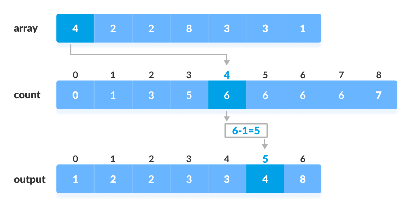
begin countSort(arr, n)
    declare a count array of max range 256.
    mark all elements of the count array as 0.

    Run a for loop from i:=0 to i:=n-1 :
      compute the count of every element present in the array and store it at ith position of the count array.

    Run a for loop from i=1 to 256 :
      Convert the count array to prefix sum array by cummulative addding of previous elements.

    declare an output array of size n for storing the sorted sequence.

    Run a for loop from j:=n-1 to 0 :
      Insert the elments in the output using the count and original array, and Decrease  the count of each element restored by 1.

    Finally run a loop from i:=0 to i:=n-1 :
      Copy the values of output array into the original array.

  [end of program]
- Time Complexity :
- Worst case time : O(n)
- Best case time : O(n)
- Average case time : O(n)
- Auxillary Space : O(n)
- In-place : No
- Stable : Yes
- Linear time sorting technique, making it faster than comparison based algorithms.
- Works for restricted inputs only for a certain range and takes extra space.
=======
-
Bucket Sort is a sorting algorithm that divides the unsorted array elements into several groups called buckets. Each bucket is then sorted by using any of the suitable sorting algorithms or recursively applying the same bucket algorithm.
-
Finally, the sorted buckets are combined to form a final sorted array.
-
In BucketSort.cpp Program, the underlying sorting technique is Insertion Sort.
-
Bucket Sort is useful when:
-
inputs are scattered within a range.
-
floating point numbers are taken as inputs.
-

The process of bucket sort can be understood as a scatter-gather approach. Here, elements are first scattered into buckets then the elements in each bucket are sorted. Finally, the elements are gathered in order. To implement Bucket Sort in C++:
-
Create an array of size 10 to input elements to sort.
-
Create a self-referential structure Node with data member to hold array element and a pointer to refer to the next node.
-
Create buckets of Node double pointer type and allocate memory to them according to the capacity assigned to each bucket.
-
Initialize the empty buckets to NULL by taking a loop.
-
Retrieve the bucket index corresponding to each array element by dividing the element value with bucket capacity, i.e., 10.
-
Using bucket index and a loop, insert array elements to the buckets of matching range.
-
Now that the buckets contain unsorted elements, Insertion Sort is applied on each bucket to sort them. Refer to Insertion Sort Algorithm.
-
Combine the sorted buckets and put them back on the original input array to form a sorted array.
  bucketSort()

    create N buckets each of which can hold a range of values

    for all the buckets
      initialize each bucket with 0 values

    for all the buckets
      put elements into buckets matching the range

    for all the buckets
      sort elements in each bucket

    gather elements from each bucket

    end bucketSort
-
Time Complexity:
-
Worst Case Complexity: O(n^2)- When there are elements of close range in the array, they are likely to be placed in the same bucket. This may result in some buckets having more number of elements than others.
- It makes the complexity depend on the sorting algorithm used to sort the elements of the bucket. The complexity becomes even worse when the elements are in reverse order. If insertion sort is used to sort elements of the bucket, then the time complexity becomes O(n^2).
-
Best Case Complexity: O(n+k)- It occurs when the elements are uniformly distributed in the buckets with a nearly equal number of elements in each bucket.
- The complexity becomes even better if the elements inside the buckets are already sorted.
- If insertion sort is used to sort elements of a bucket then the overall complexity in the best case will be linear ie. O(n+k).
- O(n) is the complexity for making the buckets and O(k) is the complexity for sorting the elements of the bucket using algorithms having linear time complexity at the best case.
-
Average Case Complexity: O(n)- It occurs when the elements are distributed randomly in the array. Even if the elements are not distributed uniformly, bucket sort runs in linear time. It holds true until the sum of the squares of the bucket sizes is linear in the total number of elements.
-
-
Space Complexity: O(n+k) -
Stable: Depends on the underlying sorting algorithm- In case of BucketSort.cpp, the underlying sorting algorithm, that is, Insertion Sort is stable, hence Bucket Sort is also stable.
-
In-place: No
-
Bucket sort allows each bucket to be processed independently. As a result, you’ll frequently need to sort much smaller arrays as a secondary step after sorting the main array.
-
For already sorted input values, it is also seen that Bucket Sort is faster than Radix Sort.
-
Bucket sort also has the advantage of being able to be used as an external sorting algorithm. If you need to sort a list that is too large to fit in memory, you may stream it through RAM, split the contents into buckets saved in external files, and then sort each file separately in RAM.
-
The problem is that if the buckets are distributed incorrectly, you may wind up spending a lot of extra effort for no or very little gain. As a result, bucket sort works best when the data is more or less evenly distributed, or when there is a smart technique to pick the buckets given a fast set of heuristics based on the input array.
-
Can’t apply it to all data types since a suitable bucketing technique is required. Bucket sort’s efficiency is dependent on the distribution of the input values, thus it’s not worth it if your data are closely grouped.In many situations, you might achieve greater performance by using a specialized sorting algorithm like radix sort, counting sort, or burst sort instead of bucket sort.
-
Bucket sort’s performance is determined by the number of buckets used, which may need some additional performance adjustment when compared to other algorithms.
- Shell sort is a special case of insertion sort. It was designed to overcome the drawbacks of insertion sort. Thus, it is more efficient than insertion sort.
- Also known as Shell's method, an in-place comparison sort. It can be seen as either a generalization of sorting by exchange or sorting by insertion.
- The method starts by sorting pairs of elements far apart from each other, then progressively reducing the gap between elements to be compared
- Sorting array by breaking it down into a number of smaller subarrays.
- Not necessary lists of contiguous elements.
- Instead, shell sort algorithm uses increment gap, to create the array of elements that are “gap” elements apart.

shellSort(array, size)

    1) Set the gap value (prefered to be arraySize / 2).
    2) Start a loop and keep dividing the gap value by 2 until it reaches less than 1 which means there is no gap.

       1- Inside the loop start another loop starting from the gap value till the end of the array.
       2- Check the number you are standing on with the other numbers that are gap value steps apart, if less than them, swap them.

end shellSort
-
Time Complexity:
- Best Complexity: O(nlog n)
- Worst Complexity: O(n2)
- Average Complexity: O(nlog n)
-
Space Complexity: O(1)
-
Stability: No
- Shell sort algorithm is only efficient for finite number of elements in an array.
- Shell sort algorithm is 5.32 x faster than bubble sort algorithm.
- Shell sort algorithm is complex in structure and bit more difficult to understand.
- Shell sort algorithm is significantly slower than the merge sort, quick sort and heap sort algorithms.
DNF Sort (Dutch National Flag Sorting) , This is the sorting method which is specially designed for only the array which contain numbers 0's 1's and 2's only.

- Initialize the
low = 0,mid = 0andhigh = size - 1. - Traverse the array from starting to last till mid is less than equal to high.
- If the element is 0 then swap the element with the element at index low and increase low and mid by 1.
- If the element is 1 then increase mid by 1.
- If the element is 2 then swap the element with the element at index high and decrease the high by 1.
-
Approach
The Array is divided into four Sections
a[1 to low-1]for zeroes and as repect to flag (red in Dutch Flag).a[low to mid-1]for ones and as repect to flag (white).a[mid to high]no change.a[high+1 to n(size)]for twos and as respect to flag (blue).
- Time Complexities
- Worst case time : O(n)
- Best case time : O(n)
- Average case time : O(n)
- Auxillary Space : O(1)
- In-place : No
- Stable : Yes
- The DNF algorithm can be extended to four, or even more colours.
- Can we used as an alternative to find two different elements
a1anda2, from the arrayasuch thata1<a2.
- Problem was restricted by allowing the inspection of the color of each element only once.
-
Cycle sort is a comparison based sorting algorithm which forces array to be factored into the number of cycles where each of them can be rotated to produce a sorted array.
-
It is an in-place and unstable sorting algorithm.
-
It is optimal in terms of number of memory writes. It minimizes the number of memory writes to sort. Each value is either written zero times, if it’s already in its correct position, or written one time to its correct position.
-
It is based on the idea that array to be sorted can be divided into cycles. Cycles can be visualized as a graph. We have n nodes and an edge directed from node i to node j if the element at i-th index must be present at j-th index in the sorted array.
Here, array elements: {30, 20, 10, 40, 60, 50}

-
An array of n distinct elements is to be considered.
-
An element a is given, index of a can be calculated by counting the number of elements that are smaller than a.
-
If the element is found to be at its correct position, simply leave it as it is.
-
Otherwise, find the correct position of a by counting the total number of elements that are less than a. where it must be present in the sorted array. The other element b which is replaced is to be moved to its correct position. This process continues until we got an element at the original position of a.
Begin
for start := 0 to n – 2 do
item := arr[start]
pos := start
for i := start + 1 to n-1 do
  if arr[i] < item then
     pos:= pos+1
done

if pos = start then
    ignore lower part, go for next iteration
while item = arr[pos] do
    pos := pos+1
done

if pos != start then
    swap arr[pos] with item
while pos != start do
    pos := start
    for i := start + 1 to n-1 do
           if arr[i] < item then
                pos:= pos+1
    done

    while item = arr[pos]
           pos := pos +1
    if item != arr[pos]
           swap arr[pos] and item
   done
  done
End
- Time Complexity: O(n^2)
- Space Complexity: O(1)
- In-place : Yes
- Stable : No
-
Cycle Sort offers the advantage of little or no additional storage.
-
It is an in-place sorting Algorithm.
-
It is optimal in terms of number of memory writes. It makes minimum number of writes to the memory and hence efficient when array is stored in EEPROM or Flash. Unlike nearly every other sort (Quick , insertion , merge sort), items are never written elsewhere in the array simply to push them out of the way of the action. Each value is either written zero times, if it's already in its correct position, or written one time to its correct position.This matches the minimal number of overwrites required for a completed in-place sort.
- It is not mostly used because it has more time complexity (i.e O(n^2)) than any other comparison sorting algorithm.